QTL Model Selection 1 Bayesian strategy 2 Markov

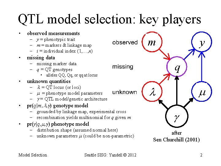
QTL model selection: key players • observed measurements – y = phenotypic trait – m = markers & linkage map – i = individual index (1, …, n) • m missing data q – missing marker data – q = QT genotypes • alleles QQ, Qq, or qq at locus • unknown quantities • pr(q|m, , ) genotype model – = QT locus (or loci) – = phenotype model parameters – = QTL model/genetic architecture – grounded by linkage map, experimental cross – recombination yields multinomial for q given m • pr(y|q, , ) phenotype model – distribution shape (assumed normal here) – unknown parameters (could be non-parametric) Model Selection Seattle SISG: Yandell © 2012 y after Sen Churchill (2001) 2

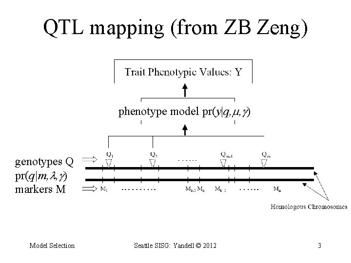
QTL mapping (from ZB Zeng) phenotype model pr(y|q, , ) genotypes Q pr(q|m, ,

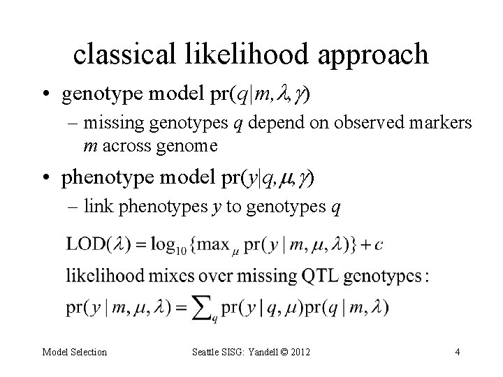
classical likelihood approach • genotype model pr(q|m, , ) – missing genotypes q depend on observed markers m across genome • phenotype model pr(y|q, , ) – link phenotypes y to genotypes q Model Selection Seattle SISG: Yandell © 2012 4

EM approach • Iterate E and M steps – expectation (E): geno prob’s pr(q|m, , ) – maximization (M): pheno model parameters • mean, effects, variance – careful attention when many QTL present • Multiple papers by Zhao-Bang Zeng and others – Start with simple initial model • Add QTL, epistatic effects sequentially Model Selection Seattle SISG: Yandell © 2012 5

classic model search • initial model from single QTL analysis • search for additional QTL • search for epistasis between pairs of QTL – Both in model? One in model? Neither? • Refine model – Update QTL positions – Check if existing QTL can be dropped • Analogous to stepwise regression Model Selection Seattle SISG: Yandell © 2012 6

comparing models (details later) • balance model fit against model complexity – want to fit data well (maximum likelihood) – without getting too complicated a model smaller model fit model miss key features estimate phenotype may be biased predict new data may be biased interpret model easier estimate effects low variance Sys. Gen: Overview Seattle SISG: Yandell © 2012 bigger model fits better no bias more complicated high variance 7

1. Bayesian strategy for QTL study • augment data (y, m) with missing genotypes q • study unknowns ( , , ) given augmented data (y, m, q) – find better genetic architectures – find most likely genomic regions = QTL = – estimate phenotype parameters = genotype means = • sample from posterior in some clever way – multiple imputation (Sen Churchill 2002) – Markov chain Monte Carlo (MCMC) • (Satagopan et al. 1996; Yi et al. 2005, 2007) Model Selection Seattle SISG: Yandell © 2012 8

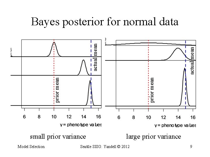
prior mean actual mean Bayes posterior for normal data small prior variance Model Selection

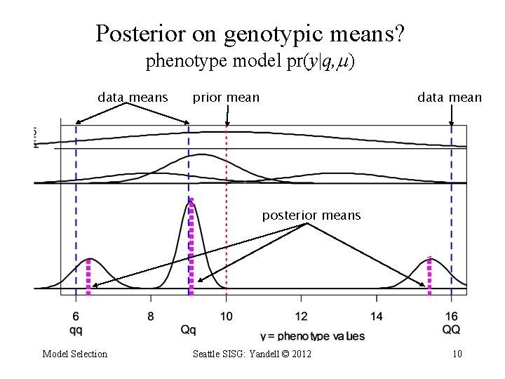
Posterior on genotypic means? phenotype model pr(y|q, ) data means prior mean data mean

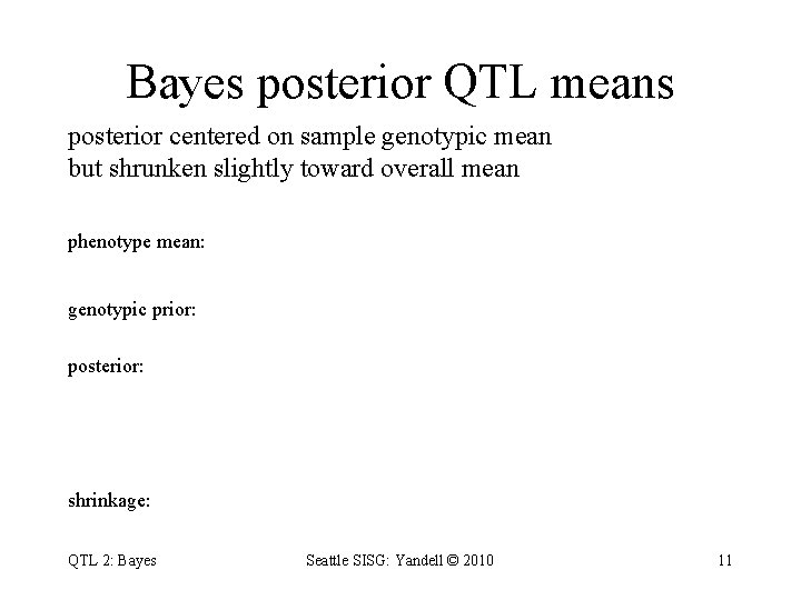
Bayes posterior QTL means posterior centered on sample genotypic mean but shrunken slightly toward overall mean phenotype mean: genotypic prior: posterior: shrinkage: QTL 2: Bayes Seattle SISG: Yandell © 2010 11

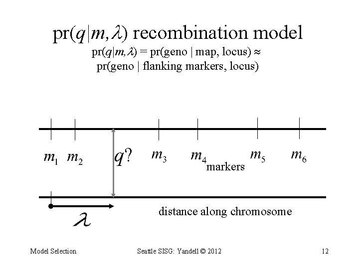
pr(q|m, ) recombination model pr(q|m, ) = pr(geno | map, locus) pr(geno | flanking

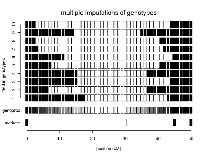
Model Selection Seattle SISG: Yandell © 2012 13

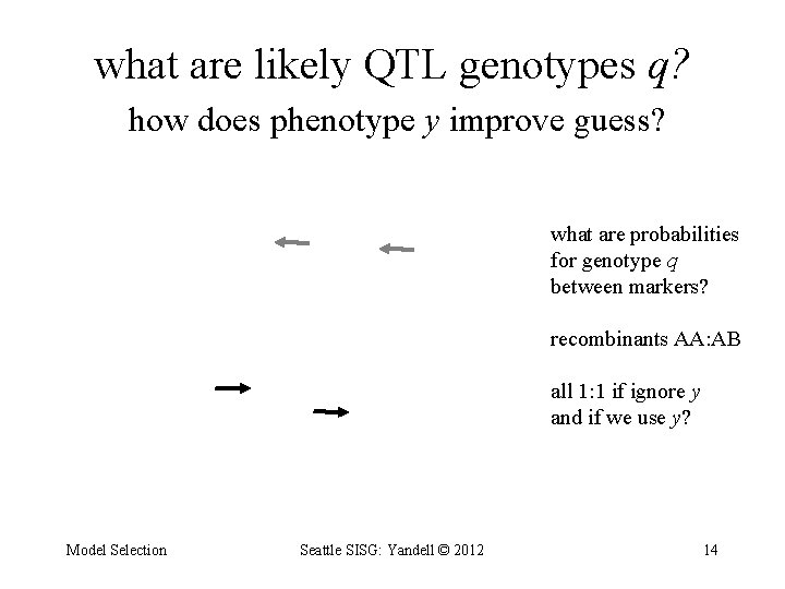
what are likely QTL genotypes q? how does phenotype y improve guess? what are probabilities for genotype q between markers? recombinants AA: AB all 1: 1 if ignore y and if we use y? Model Selection Seattle SISG: Yandell © 2012 14

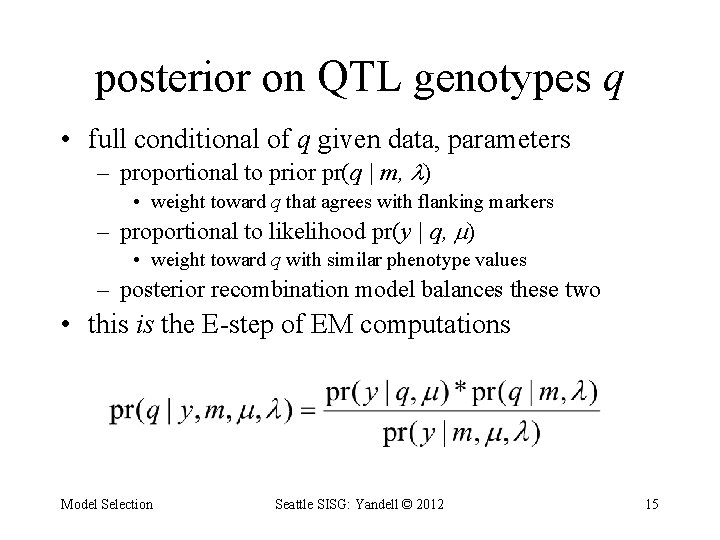
posterior on QTL genotypes q • full conditional of q given data, parameters – proportional to prior pr(q | m, ) • weight toward q that agrees with flanking markers – proportional to likelihood pr(y | q, ) • weight toward q with similar phenotype values – posterior recombination model balances these two • this is the E-step of EM computations Model Selection Seattle SISG: Yandell © 2012 15

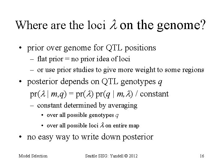
Where are the loci on the genome? • prior over genome for QTL positions – flat prior = no prior idea of loci – or use prior studies to give more weight to some regions • posterior depends on QTL genotypes q pr( | m, q) = pr( ) pr(q | m, ) / constant – constant determined by averaging • over all possible genotypes q • over all possible loci on entire map • no easy way to write down posterior Model Selection Seattle SISG: Yandell © 2012 16

what is the genetic architecture ? • which positions correspond to QTLs? – priors on loci (previous slide) • which QTL have main effects? – priors for presence/absence of main effects • same prior for all QTL • can put prior on each d. f. (1 for BC, 2 for F 2) • which pairs of QTL have epistatic interactions? – prior for presence/absence of epistatic pairs • depends on whether 0, 1, 2 QTL have main effects • epistatic effects less probable than main effects Model Selection Seattle SISG: Yandell © 2012 17

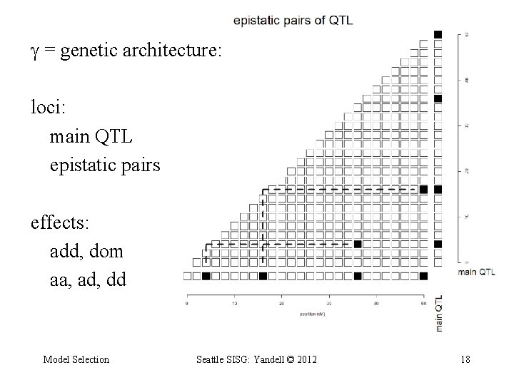
= genetic architecture: loci: main QTL epistatic pairs effects: add, dom aa, ad,

Bayesian priors & posteriors • augmenting with missing genotypes q – prior is recombination model – posterior is (formally) E step of EM algorithm • sampling phenotype model parameters – prior is “flat” normal at grand mean (no information) – posterior shrinks genotypic means toward grand mean – (details for unexplained variance omitted here) • sampling QTL loci – prior is flat across genome (all loci equally likely) • sampling QTL genetic architecture model – number of QTL • prior is Poisson with mean from previous IM study – genetic architecture of main effects and epistatic interactions • priors on epistasis depend on presence/absence of main effects Model Selection Seattle SISG: Yandell © 2012 19

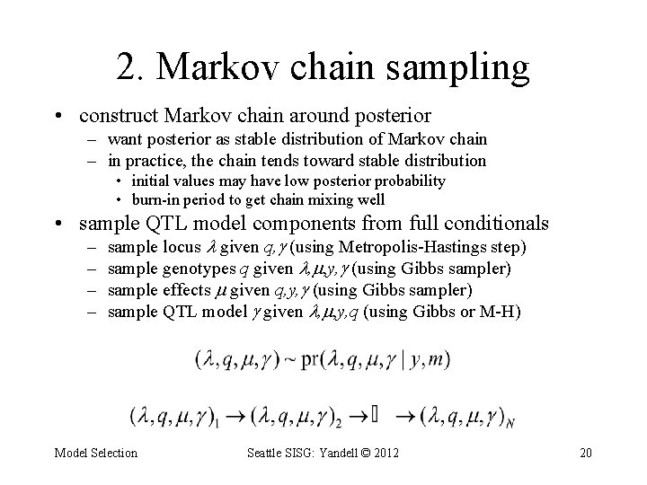
2. Markov chain sampling • construct Markov chain around posterior – want posterior as stable distribution of Markov chain – in practice, the chain tends toward stable distribution • initial values may have low posterior probability • burn-in period to get chain mixing well • sample QTL model components from full conditionals – – sample locus given q, (using Metropolis-Hastings step) sample genotypes q given , , y, (using Gibbs sampler) sample effects given q, y, (using Gibbs sampler) sample QTL model given , , y, q (using Gibbs or M-H) Model Selection Seattle SISG: Yandell © 2012 20

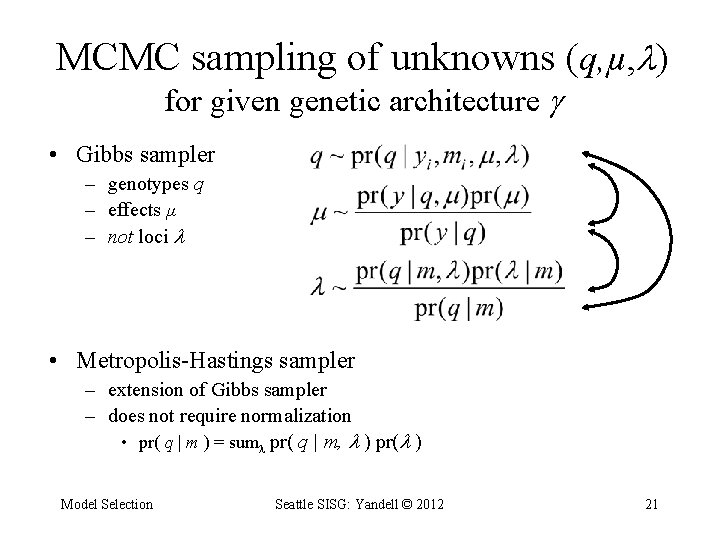
MCMC sampling of unknowns (q, µ, ) for given genetic architecture • Gibbs sampler – genotypes q – effects µ – not loci • Metropolis-Hastings sampler – extension of Gibbs sampler – does not require normalization • pr( q | m ) = sum pr( q | m, ) pr( ) Model Selection Seattle SISG: Yandell © 2012 21

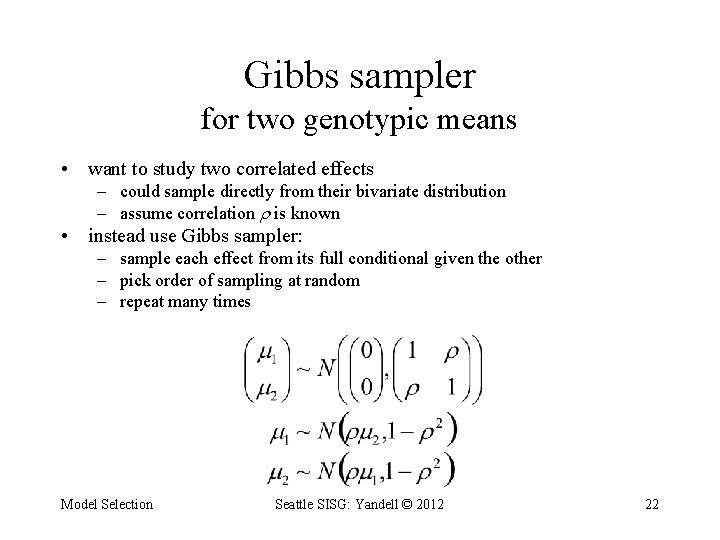
Gibbs sampler for two genotypic means • want to study two correlated effects – could sample directly from their bivariate distribution – assume correlation is known • instead use Gibbs sampler: – sample each effect from its full conditional given the other – pick order of sampling at random – repeat many times Model Selection Seattle SISG: Yandell © 2012 22

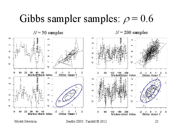
Gibbs sampler samples: = 0. 6 N = 200 samples N = 50 samples

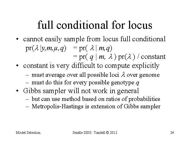
full conditional for locus • cannot easily sample from locus full conditional pr( |y, m, µ, q) = pr( | m, q) = pr( q | m, ) pr( ) / constant • constant is very difficult to compute explicitly – must average over all possible loci over genome – must do this for every possible genotype q • Gibbs sampler will not work in general – but can use method based on ratios of probabilities – Metropolis-Hastings is extension of Gibbs sampler Model Selection Seattle SISG: Yandell © 2012 24

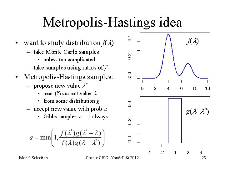
Metropolis-Hastings idea • want to study distribution f( ) – take Monte Carlo samples • unless too complicated – take samples using ratios of f • Metropolis-Hastings samples: – propose new value * • near (? ) current value • from some distribution g – accept new value with prob a • Gibbs sampler: a = 1 always Model Selection Seattle SISG: Yandell © 2012 g( – *) 25

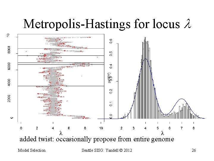
Metropolis-Hastings for locus added twist: occasionally propose from entire genome Model Selection Seattle SISG:

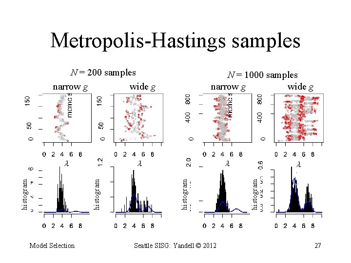
Metropolis-Hastings samples N = 200 samples narrow g wide g Model Selection Seattle SISG:

3. sampling genetic architectures • search across genetic architectures of various sizes – allow change in number of QTL – allow change in types of epistatic interactions • methods for search – reversible jump MCMC – Gibbs sampler with loci indicators • complexity of epistasis – Fisher-Cockerham effects model – general multi-QTL interaction & limits of inference Model Selection Seattle SISG: Yandell © 2012 28

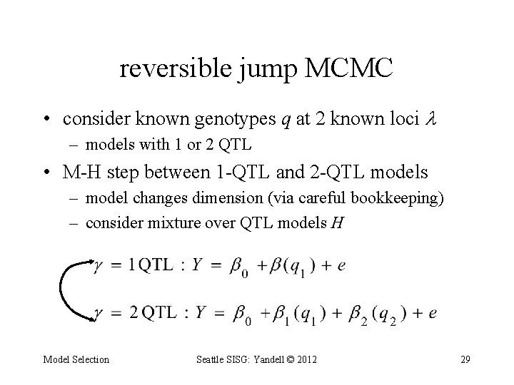
reversible jump MCMC • consider known genotypes q at 2 known loci – models with 1 or 2 QTL • M-H step between 1 -QTL and 2 -QTL models – model changes dimension (via careful bookkeeping) – consider mixture over QTL models H Model Selection Seattle SISG: Yandell © 2012 29

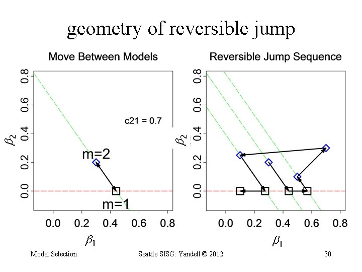
2 2 geometry of reversible jump 1 Model Selection Seattle SISG: Yandell ©

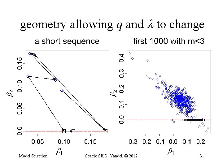
2 2 geometry allowing q and to change Model Selection 1 Seattle SISG:

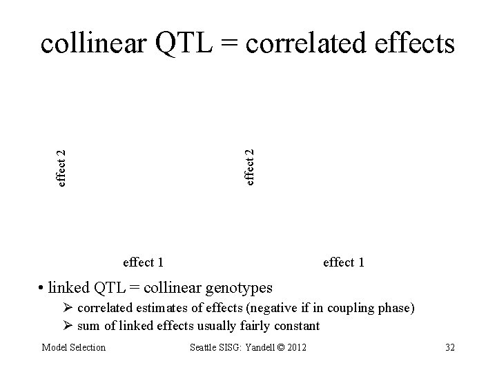
effect 2 collinear QTL = correlated effects effect 1 • linked QTL = collinear genotypes Ø correlated estimates of effects (negative if in coupling phase) Ø sum of linked effects usually fairly constant Model Selection Seattle SISG: Yandell © 2012 32

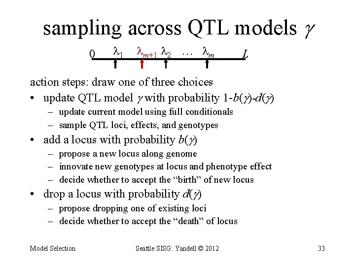
sampling across QTL models 0 1 m+1 2 … m L action steps: draw one of three choices • update QTL model with probability 1 -b( )-d( ) – update current model using full conditionals – sample QTL loci, effects, and genotypes • add a locus with probability b( ) – propose a new locus along genome – innovate new genotypes at locus and phenotype effect – decide whether to accept the “birth” of new locus • drop a locus with probability d( ) – propose dropping one of existing loci – decide whether to accept the “death” of locus Model Selection Seattle SISG: Yandell © 2012 33

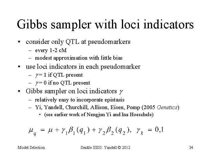
Gibbs sampler with loci indicators • consider only QTL at pseudomarkers – every 1 -2 c. M – modest approximation with little bias • use loci indicators in each pseudomarker – = 1 if QTL present – = 0 if no QTL present • Gibbs sampler on loci indicators – relatively easy to incorporate epistasis – Yi, Yandell, Churchill, Allison, Eisen, Pomp (2005 Genetics) • (see earlier work of Nengjun Yi and Ina Hoeschele) Model Selection Seattle SISG: Yandell © 2012 34

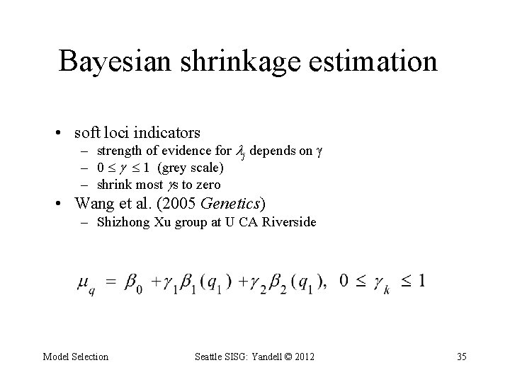
Bayesian shrinkage estimation • soft loci indicators – strength of evidence for j depends on – 0 1 (grey scale) – shrink most s to zero • Wang et al. (2005 Genetics) – Shizhong Xu group at U CA Riverside Model Selection Seattle SISG: Yandell © 2012 35

other model selection approaches • include all potential loci in model • assume “true” model is “sparse” in some sense • Sparse partial least squares – Chun, Keles (2009 Genetics; 2010 JRSSB) • LASSO model selection – Foster (2006); Foster Verbyla Pitchford (2007 JABES) – Xu (2007 Biometrics); Yi Xu (2007 Genetics) – Shi Wahba Wright Klein (2008 Stat & Infer) Model Selection Seattle SISG: Yandell © 2012 36

4. criteria for model selection balance fit against complexity • classical information criteria – penalize likelihood L by model size | | – IC = – 2 log L( | y) + penalty( ) – maximize over unknowns • Bayes factors – marginal posteriors pr(y | ) – average over unknowns Model Selection Seattle SISG: Yandell © 2012 37

classical information criteria • start with likelihood L( | y, m) – measures fit of architecture ( ) to phenotype (y) • given marker data (m) – genetic architecture ( ) depends on parameters • have to estimate loci (µ) and effects ( ) • complexity related to number of parameters – | | = size of genetic architecture • BC: | | = 1 + n. qtl(n. qtl - 1) = 1 + 4 + 12 = 17 • F 2: | | = 1 + 2 n. qtl +4 n. qtl(n. qtl - 1) = 1 + 8 + 48 = 57 Model Selection Seattle SISG: Yandell © 2012 38

classical information criteria • construct information criteria – balance fit to complexity – Akaike AIC = – 2 log(L) + 2 | | – Bayes/Schwartz BIC = – 2 log(L) + | | log(n) – Broman BIC = – 2 log(L) + | | log(n) – general form: IC = – 2 log(L) + | | D(n) • compare models – hypothesis testing: designed for one comparison • 2 log[LR( 1, 2)] = L(y|m, 2) – L(y|m, 1) – model selection: penalize complexity • IC( 1, 2) = 2 log[LR( 1, 2)] + (| 2| – | 1|) D(n) Model Selection Seattle SISG: Yandell © 2012 39

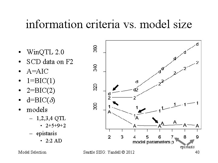
information criteria vs. model size • • Win. QTL 2. 0 SCD data on F 2 A=AIC 1=BIC(1) 2=BIC(2) d=BIC( ) models – 1, 2, 3, 4 QTL • 2+5+9+2 – epistasis • 2: 2 AD epistasis Model Selection Seattle SISG: Yandell © 2012 40

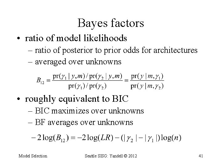
Bayes factors • ratio of model likelihoods – ratio of posterior to prior odds for architectures – averaged over unknowns • roughly equivalent to BIC – BIC maximizes over unknowns – BF averages over unknowns Model Selection Seattle SISG: Yandell © 2012 41

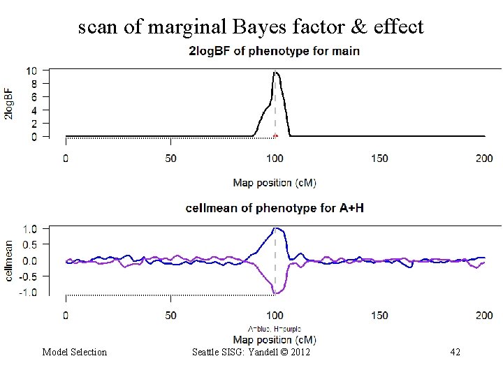
scan of marginal Bayes factor & effect Model Selection Seattle SISG: Yandell © 2012

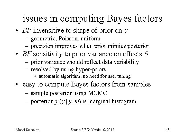
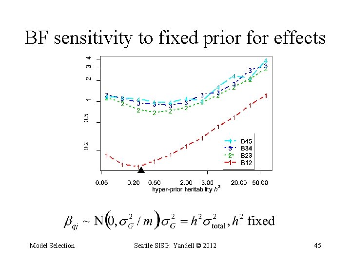
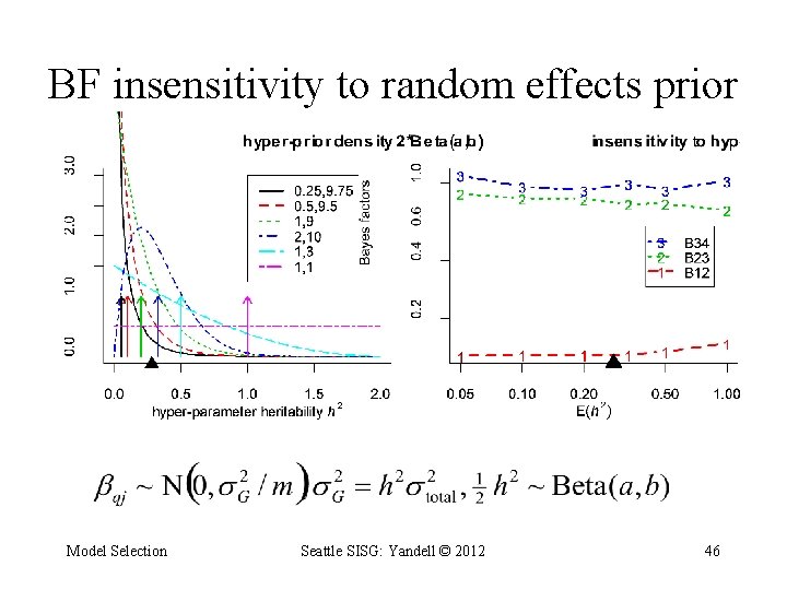
issues in computing Bayes factors • BF insensitive to shape of prior on – geometric, Poisson, uniform – precision improves when prior mimics posterior • BF sensitivity to prior variance on effects – prior variance should reflect data variability – resolved by using hyper-priors • automatic algorithm; no need for user tuning • easy to compute Bayes factors from samples – sample posterior using MCMC – posterior pr( | y, m) is marginal histogram Model Selection Seattle SISG: Yandell © 2012 43

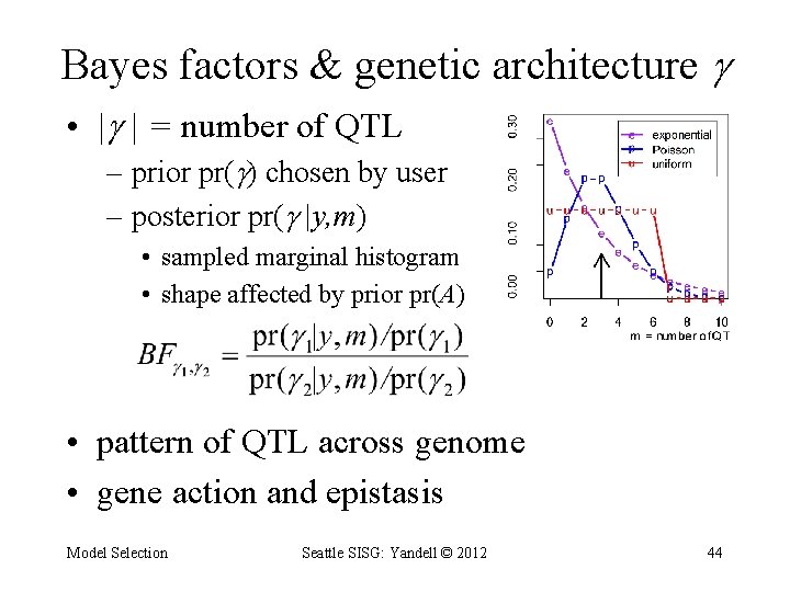
Bayes factors & genetic architecture • | | = number of QTL – prior pr( ) chosen by user – posterior pr( |y, m) • sampled marginal histogram • shape affected by prior pr(A) • pattern of QTL across genome • gene action and epistasis Model Selection Seattle SISG: Yandell © 2012 44