qatomic data type physical data type qstructure data


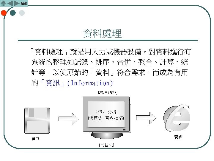

或稱為 實質資料型態(physical data type) q結構型資料型態(structure data type)或 稱為虛擬資料型態(virtual data type)")

=Sc+Sp(I) l l Sc (Fix space requirement) including instruction space, constants,")
=Tc+Tp(I) l l Tc (Fix time requirement) compile time, Tc is")
")
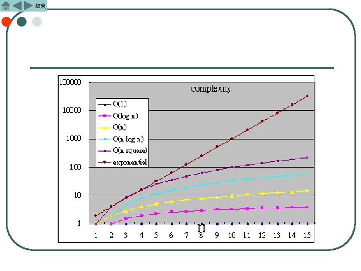
)可視為某演算法在電腦中所需執行時間不會超 過某一常數倍的g(n),也就是說當某演算法的空間或 時間複雜度(space or time complexity)為O(g(n))(讀成big -oh of g(n)或order is g(n))。")
:稱為常數 (constant) O(log 2 n):稱為 (logarithmic) O(log 22")
的介紹 l Ω也是一種複雜度的漸近表示法,如果說Big-oh是執 行時間量度的最壞情況,那Ω就是執行時間量度的最 好狀況。以下是Ω的定義: l Definition: The function f(n) is said to")
的介紹 l 是一種比Big-O與Ω更精確複雜度的漸近表示法。定 義如下: Definition: The function f(n) is θ(g(n)) iff there exists")
, ∵ 3")
: addup values of n elements in an array called list.")
: use step count instead of execution time. 1. on-line step")
![結束 2. Tabular method void add( int a[ ][ ], int b[ ][ ],](https://slidetodoc.com/presentation_image_h2/5fdf6d73f35063d996b6874789227570/image-33.jpg "結束 2. Tabular method void add( int a[ ][ ], int b[ ][ ],")


- Slides: 35
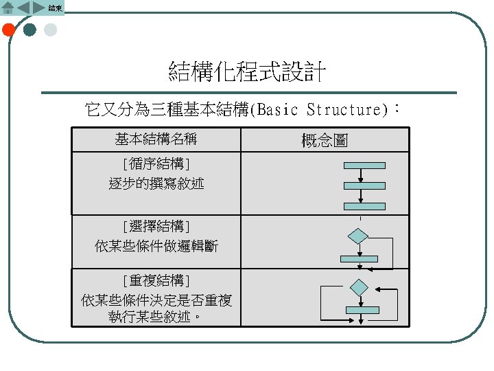
結束 資料儲存層次的分類 q基本資料型態(atomic data type)或稱為 實質資料型態(physical data type) q結構型資料型態(structure data type)或 稱為虛擬資料型態(virtual data type) q抽象資料型態(Abstract Data Type:ADT)
結束 4. 演算法的效能分析 Given a problem, there may be several possible implementations. Efficiency is the most important consideration including time and space. l Complexity Theory– to estimate the time and space needed for a program. It’s machine independent. l Space Complexity of a program – the amount of memory space needed to complete a program. l Time Complexity of a program – the amount of computation (computer) time needed to complete a program.
結束 Space Complexity S(p)=Sc+Sp(I) l l Sc (Fix space requirement) including instruction space, constants, simple variables, and fix-size structures. The Sc is independent of the number and size of inputs and outputs. e. g. int i, sum=0, A[100]; Sp(I) (Variable space requirement) depends on a particular instance I of a problem. Instance I may be a function of number, size, or values of inputs and outputs. e. g. int *n; //score list of a course
結束 Time Complexity T(p)=Tc+Tp(I) l l Tc (Fix time requirement) compile time, Tc is independent of any instance of the problem. Tp(I) (Variable time requirement) execution time, depends on a particular instance I of a problem. e. g. matrix multiplication C[ ] =A[ ] *B[ ] (0, 0) 0, 1 0, 2 0, 3 0, n 0, 0 1, 0 2, 0 n, 0 (n*) + (n+) => 2 n 2 n* n*n + an 2+bn+c => 2 n 3 +an 2+bn+c
結束 Asymptotic Notations - for measuring space and time complexities l l l O(Big-oh) Ω(omega) θ(theta)
結束 Big-oh的介紹 l O(g(n))可視為某演算法在電腦中所需執行時間不會超 過某一常數倍的g(n),也就是說當某演算法的空間或 時間複雜度(space or time complexity)為O(g(n))(讀成big -oh of g(n)或order is g(n))。 l Definition: The function f(n) is said to be of order at most g(n) if there are positive constants c and n 0 such that f(n)<=cg(n) for all n, n>=n 0. l Therefore, “Big oh” is the smallest upper bound of f(n).
結束 常見的Big-oh有下列幾種: l l l l O(1):稱為常數 (constant) O(log 2 n):稱為 (logarithmic) O(log 22 n):稱為 (log squared) O(n):稱為線性 (linear) O(nlog 2 n):稱為n log n O(n 2):稱為平方 (quadratic) O(n 3):稱為立方 (cubic) O(2 n):稱為指數 (exponential)
結束 Ω(omega)的介紹 l Ω也是一種複雜度的漸近表示法,如果說Big-oh是執 行時間量度的最壞情況,那Ω就是執行時間量度的最 好狀況。以下是Ω的定義: l Definition: The function f(n) is said to be of order at least g(n) if there are positive constants c and n 0 such that f(n)>=cg(n) for all n, n>=n 0. l Therefore, “Big oh” is the largest lower bound of f(n).
結束 θ(theta)的介紹 l 是一種比Big-O與Ω更精確複雜度的漸近表示法。定 義如下: Definition: The function f(n) is θ(g(n)) iff there exists positive constants c 1, c 2 and n 0 , such that c 1 g(n) <=f(n)<= c 2 g(n) for all n, n>=n 0. l Therefore, “θ” is both the smallest upper bound and the l greatest lower bound of f(n).
結束 Examples for asymptotic notations 1. 3 n + 2 = Ο(n), ∵ 3 n +2 ≦ 4 n, for all n ≧ 2, c = 4. 2. 3 n + 3 = Ο(n), ∵ 3 n +3 ≦ 4 n, for all n ≧ 3, c = 4. 3. 3 n + 3 = Ο(n 2), ∵ 3 n +2 ≦ 3 n 2, for all n ≧ 2, c = 3. (2) is correct. (3) is wrong. “Big oh“ should be a smaller function of n. 4. 10 n 2 + 4 n +2 = Ο(n 2), ∵ 10 n 2 + 4 n +2≦ 11 n 2, for all n ≧ 5, c = 11. 5. 6.2 n + n 2 = Ο(2 n), ∵ 6.2 n + nn≦ 7.2 n, for all n ≧ 4, c = 7. 6. 3 n +3 = Ω(n), ∵ 3 n +3 ≧ 3 n, for all n ≧ 1, c = 3. 7. 3 n +3 = Ω(1), ∵ 3 n +3 ≧ 3, for all n ≧ 1, c = 3. (6) is correct. (7) is wrong. “Omega” should be a larger function of n. 8. 3 n +2 = Θ(n) ∵ 3 n≦ 3 n +2 ≦ 4 n, for all n ≧ 2, c 1 = 3, c 2= 4 , and n 0= 2.
結束 Example for S(p): addup values of n elements in an array called list. main( ) float addup(float list[ ], int n) { { float list[n], temp = 0. 0; float temp = 0. 0; int i; for( i=0; i < n; i++) temp += list[i]; return temp; } } Smain(n) = c + n = O(n) Saddup(n) = c = O(1) Other languages may need to pass the whole array, but addup passes only addresses of the 1‘st element and the size of array.
結束 Example for T(p): use step count instead of execution time. 1. on-line step count float sum(float list[ ], int n) /* calculate the sum of an array */ { float tmp=0. 0; count ++; /* tmp assignment */ int i; for ( i=0; i <n; i++ ){ count++; /* for loop */ tmp+=list[i]; count++; * adding up */ } count++; /* last time to check for loop and fails */ return tmp; count++; /* for return */ } => step count = 2*n +3 => Tsum(n) = O(n)
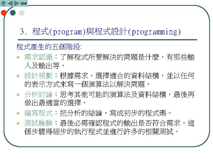
結束 2. Tabular method void add( int a[ ][ ], int b[ ][ ], int c[ ][ ], int row, int col) { Step per exec. freq. total int i, j; 0 0 0 for ( i=0; i<row; I++) 1 row +1 row+1 for ( j=0; j<col; j++) 1 row*(col+1) row*col + row c[i][j] = a[i][j]+b[i][j]; 1 row*col } In total, we have step count = 2 row*col +2 row +1. => Tadd(row, col) = O(row*col) Thus, if row >>col, one may want to exchange i and j to reduce the step count and execution time.
結束 3. Execution time Measurement #include <time. h> 1. Clock 2. Time Before execution, use start = clock(); start = time(NULL); After execution, use stop = clock(); stop = time(NULL); Type return clock_t time_t result in sec. (stop - start)/ CLK_TCK; difftime(stop, start); When measuring the execution of a program, we have CLK_TCK= 18. 2, beginclk = 66, stopclk = 193, diffclk = 127, time = 6. 98 begintime=825316157, stoptime = 825316164, difftime = 7 Note: 1. The time is begin at around 1970. 2. Use %ld to print out a long integer
結束 trade-off between program space and execution time Example: Two ways to interchange two elements, using a functions or a macro 1. using a function 2. using a macro void swap (int *x, int *y) #define swap(a, b, t) ((t)=(a), (a)=(b), (b)=(t)) { … int temp; swap(p, q, temp); temp = *x; … *x = *y; Disadv: duplicated macros may takes lots of space. *y = temp; Adv: no calls & returns, execution time is reduced. } Adv: single copy of function => save space. Disadv: calls & returns => waste time. Therefore, a careful evaluation of the trade-offs among various aspects before the implementation of a solution is important.