Python for Data Science https github comjakevdpPython Data

Python for Data Science https: //github. com/jakevdp/Python. Data. Sci ence. Handbook

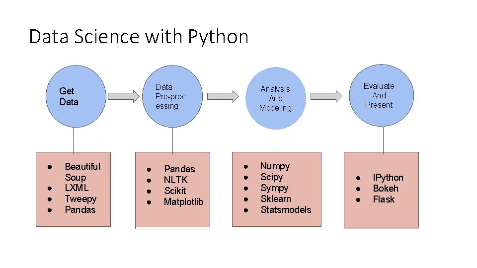
Data Science with Python Data Pre-proc essing Get Data ● ● Beautiful Soup LXML Tweepy Pandas ● ● Pandas NLTK Scikit Matplotlib Evaluate And Present Analysis And Modeling ● ● ● Numpy Scipy Sympy Sklearn Statsmodels ● ● ● IPython Bokeh Flask

IPython • Interactive Python started in 2001 as an enhanced Python interpreter • Developed by Fernando Perez as “Tools for the entire life cycle of research computing” • If Python is Engine, IPython as the interactive control panel. • Closely tied with the Jupyter project which provides browser based notebook • Two modes • IPython shell (Anaconda prompt -> Ipython) • Jupyter notebook (Anaconda prompt -> jupyter ntoebook)

IPython features • Refer to online notebooks: • https: //github. com/jakevdp/Python. Data. Science. Handbook/blob/master/note books/01. 00 -IPython-Beyond-Normal-Python. ipynb

Data as numbers • Datasets can come from a wide range of sources and formats • E. g. documents, images, sound clips, numerical measurements • Data is fundamentally array of numbers • Digital images are 2 D arrays of numbers representing pixel brightness across the area • Sound clips are 1 D arrays of intensity versus time • Text can be converted in various ways into numerical representations • First step in making data analyzable is to transform it into arrays of numbers • Both, Num. Py and Pandas package efficiently store and manipulate numerical arrays

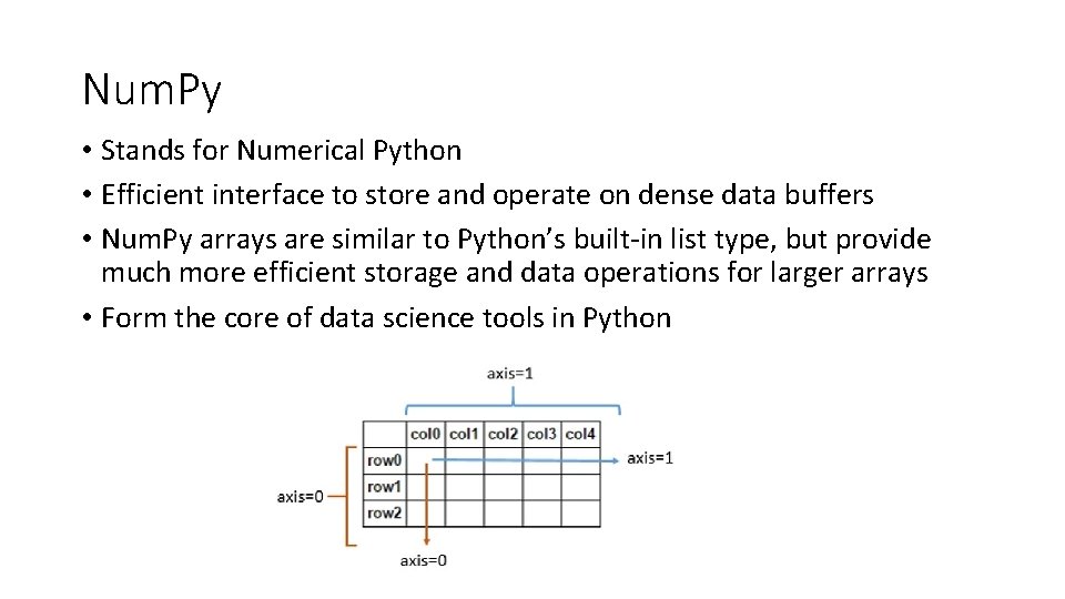
Num. Py • Stands for Numerical Python • Efficient interface to store and operate on dense data buffers • Num. Py arrays are similar to Python’s built-in list type, but provide much more efficient storage and data operations for larger arrays • Form the core of data science tools in Python

Num. Py features • Refer to online notebooks: • https: //github. com/jakevdp/Python. Data. Science. Handbook/blob/8 a 34 a 4 f 653 b dbdc 01415 a 94 dc 20 d 4 e 9 b 97438965/notebooks/02. 00 -Introduction-to. Num. Py. ipynb

Pandas • Built on top of Num. Py and provides efficient implementation of a Data. Frame • Data. Frame is multi-dimensional array with attached row and column labels • Data. Frame may contain data with heterogeneous types and/or missing data • Provides a number of powerful data operations using Series and Data. Frame objects

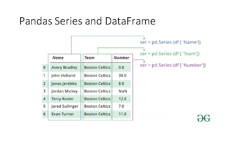
Pandas Series and Data. Frame

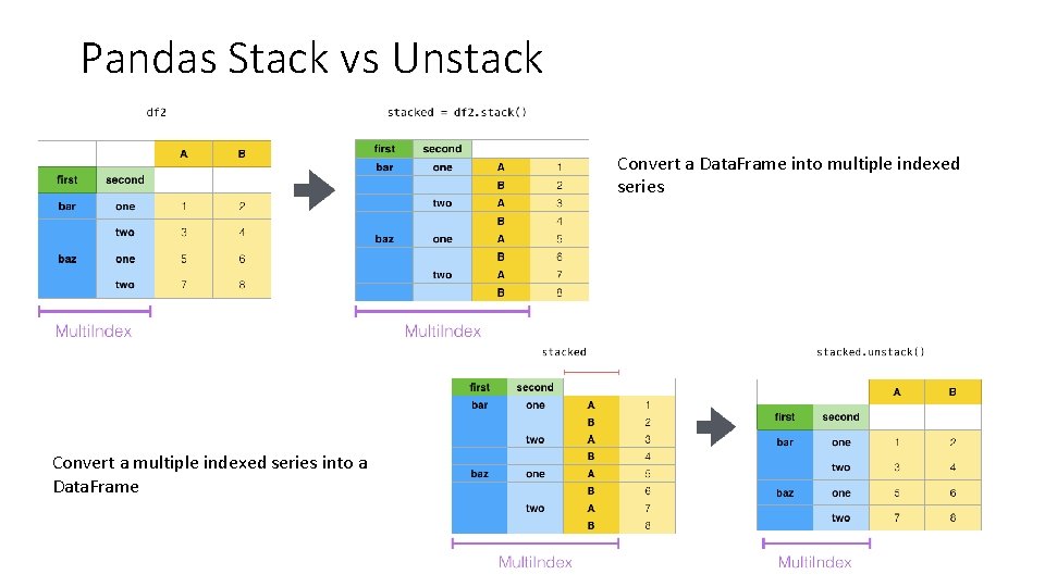
Pandas Stack vs Unstack Convert a Data. Frame into multiple indexed series Convert a multiple indexed series into a Data. Frame

Pandas features • Refer to online notebooks: • https: //jakevdp. github. io/Python. Data. Science. Handbook/03. 00 -introductionto-pandas. html

Practice exercises for Midterm 2 • Num. Py exercises: https: //www. w 3 resource. com/pythonexercises/numpy/index. php • Pandas exercises: https: //www. w 3 resource. com/pythonexercises/pandas/index. php • I will try to come up with some exercises (but keep practicing above).

Sci. Kit Learn • Provides efficient implementation of a large number of machine learning algorithms • Clean, uniform, streamlined API along with online documentation • Understand Scikit-Learn for one type of model and switch to other model effortlessly

Sci. Kit Learn – Steps in using the API • Choose a class of model by importing the appropriate estimator class from Scikit-Learn. • Choose model hyperparameters by instantiating this class with desired values. • Arrange data into a features matrix and target vector following the discussion above. • Fit the model to your data by calling the fit() method of the model instance. • Apply the Model to new data: • For supervised learning, often we predict labels for unknown data using the predict() method. • For unsupervised learning, we often transform or infer properties of the data using the transform() or predict() method.

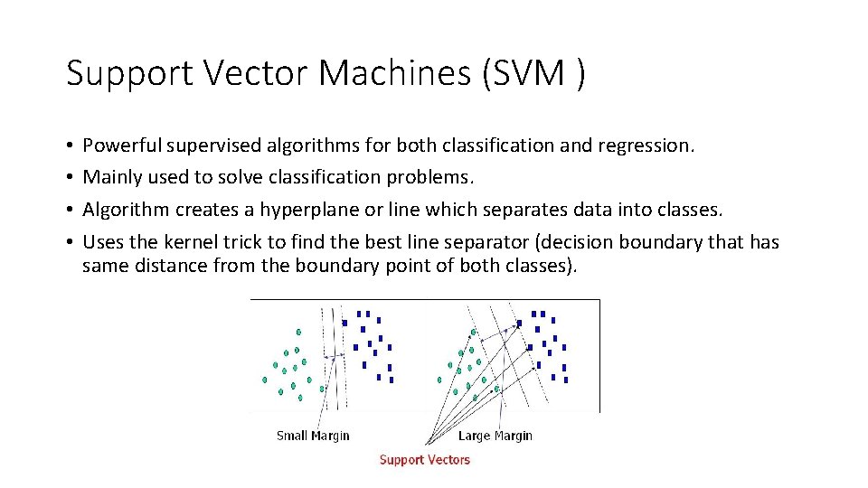
Support Vector Machines (SVM ) • • Powerful supervised algorithms for both classification and regression. Mainly used to solve classification problems. Algorithm creates a hyperplane or line which separates data into classes. Uses the kernel trick to find the best line separator (decision boundary that has same distance from the boundary point of both classes).

Difference Between SVM and Logistic Regression • SVM tries to finds the “best” margin that separates the classes and this reduces the risk of error on the data • Logistic regression can have different decision boundaries with different weights that are near the optimal point. • SVM works well with unstructured and semi-structured data like text and images. • Logistic regression works with already identified independent variables.

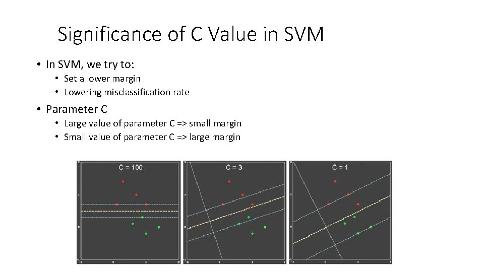
Significance of C Value in SVM • In SVM, we try to: • Set a lower margin • Lowering misclassification rate • Parameter C • Large value of parameter C => small margin • Small value of parameter C => large margin

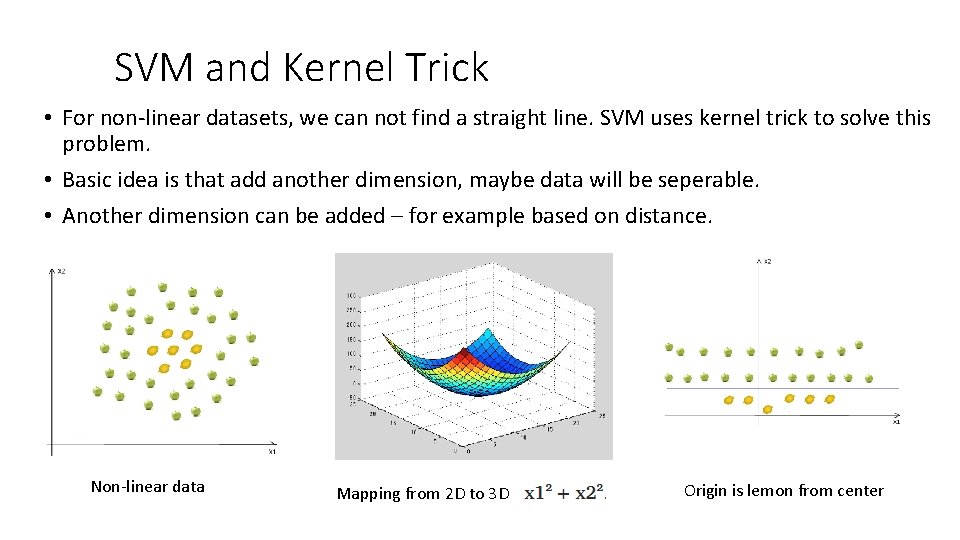
SVM and Kernel Trick • For non-linear datasets, we can not find a straight line. SVM uses kernel trick to solve this problem. • Basic idea is that add another dimension, maybe data will be seperable. • Another dimension can be added – for example based on distance. Non-linear data Mapping from 2 D to 3 D Origin is lemon from center

SVM and Kernel Trick • Few types of kernels: • Polynomial kernel • Used for image processing • d is degree of polynomial • Gaussian kernel • General purpose kernel • Gaussian Radial Basis Function (RBF) • General purpose kernel • Some SVM links for reference: • https: //towardsdatascience. com/svm-and-kernel-svm-fed 02 bef 1200 • https: //data-flair. training/blogs/svm-kernel-functions/ • https: //medium. com/axum-labs/logistic-regression-vs-support-vector-machines-svm-c 335610 a 3 d 16

Decision Trees and Random Forests • Random forests are an example of an ensemble method • Relies on aggregating the results of an ensemble of simple estimators • A majority vote among a number of estimators can end up being better than an individual estimator

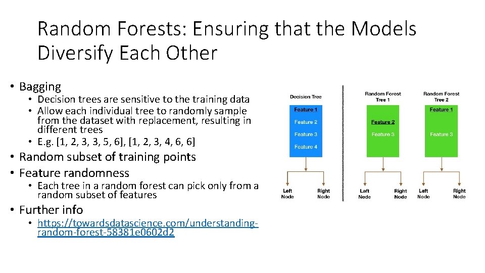
Random Forests: Ensuring that the Models Diversify Each Other • Bagging • Decision trees are sensitive to the training data • Allow each individual tree to randomly sample from the dataset with replacement, resulting in different trees • E. g. [1, 2, 3, 3, 5, 6], [1, 2, 3, 4, 6, 6] • Random subset of training points • Feature randomness • Each tree in a random forest can pick only from a random subset of features • Further info • https: //towardsdatascience. com/understandingrandom-forest-58381 e 0602 d 2

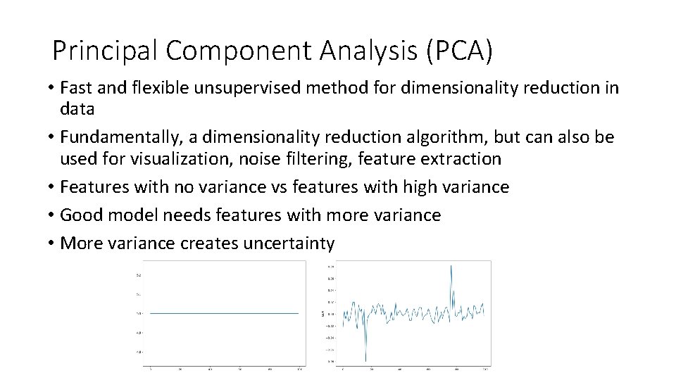
Principal Component Analysis (PCA) • Fast and flexible unsupervised method for dimensionality reduction in data • Fundamentally, a dimensionality reduction algorithm, but can also be used for visualization, noise filtering, feature extraction • Features with no variance vs features with high variance • Good model needs features with more variance • More variance creates uncertainty

Capturing Signal with Principal Components • Given data with 10, 000 features and 5, 000 observations is a terrible idea as it will result in massively overfit model • The ideal set of features should have following three properties: • High variance (contain a lot of potential signal – useful information) • Uncorrelated (Highly correlated features are less useful) • Require low number of features • PCA creates a set of principal components that are rank ordered by variance, uncorrelated and low in number • PCA finds strongest underlying trend in the feature set

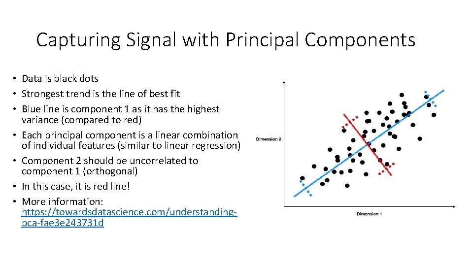
Capturing Signal with Principal Components • Data is black dots • Strongest trend is the line of best fit • Blue line is component 1 as it has the highest variance (compared to red) • Each principal component is a linear combination of individual features (similar to linear regression) • Component 2 should be uncorrelated to component 1 (orthogonal) • In this case, it is red line! • More information: https: //towardsdatascience. com/understandingpca-fae 3 e 243731 d

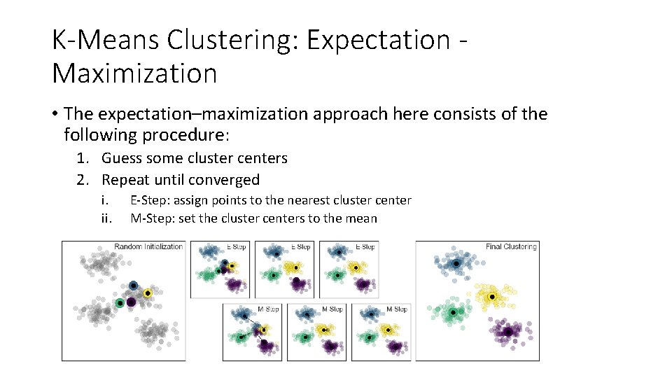
K-Means Clustering: Expectation Maximization • The expectation–maximization approach here consists of the following procedure: 1. Guess some cluster centers 2. Repeat until converged i. ii. E-Step: assign points to the nearest cluster center M-Step: set the cluster centers to the mean

K-Means Clustering: Spectral Clustering K-Means clustering is limited to linear cluster boundaries K-Means fails to find clusters with complicated geometries Solution: use approach similar to kernel tricks in SVM E. g. Spectral. Clustering uses graph of nearest neighbors to compute higherdimensional representation and assign labels using K-Means • More details: https: //towardsdatascience. com/spectral-clustering-aba 2640 c 0 d 5 b • •