Python as a data science platform for air

Python as a data science platform for air quality studies Andy Lewin Scott Hamilton Nicola Masey © Ricardo plc 2017

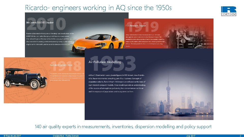
Ricardo- engineers working in AQ since the 1950 s 140 air quality experts in measurements, inventories, dispersion modelling and policy support © Ricardo plc 2017 Unclassified - Public Domain July 2017 2

Topics for this presentation Introduction • Python as a data science platform for air quality studies • Some advantages of using python for air quality science • Key libraries we use in our work Examples of practical application • Processing of millions of observation based records • Grouping processes into larger workflows or applications • Bringing it all together into ‘software’ • Try to give some insights from our experience in adopting python for our work © Ricardo plc 2017 Unclassified - Public Domain July 2017 3

Ricardo Energy & Environment Scottish Team Python Users: Scott Hamilton Nicola Masey Andy Lewin © Ricardo plc 2017 Unclassified - Public Domain July 2017 4

Introduction Challenges • Data is in abundance, but there are barriers to unlocking its latent potential • Huge volumes of data present a data management challenge to air quality practitioners e. g. – Emission source activity observations – Air quality observations – Meteorological measurements • This can make it difficult to extract insights with which to aid decision makers • With such volumes of data how will we ever use it to extract knowledge? Solution • Python's many numerical and statistical libraries (other languages are available!) • Some neat programming backed up by domain knowledge • Simple but powerful solutions can be written in a few lines of code • Getting what you want from data, and only what you want © Ricardo plc 2017 Unclassified - Public Domain July 2017 5

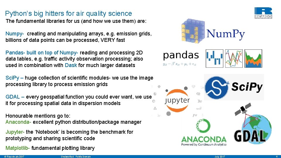
Python’s big hitters for air quality science The fundamental libraries for us (and how we use them) are: Numpy- creating and manipulating arrays, e. g. emission grids, billions of data points can be processed, VERY fast Pandas- built on top of Numpy- reading and processing 2 D data tables, e. g. traffic activity observation processing; also used in combination with Dask for much larger datasets Sci. Py – huge collection of scientific modules- we use the image processing library to process emission grids GDAL – every geospatial function you could ever want, we use it for processing spatial data in dispersion models Honourable mentions go to: Anaconda- excellent python distribution/package manager Jupyter- the ‘Notebook’ is becoming the benchmark for prototyping and sharing scientific code Matplotlib- fundamental plotting library © Ricardo plc 2017 Unclassified - Public Domain July 2017 6

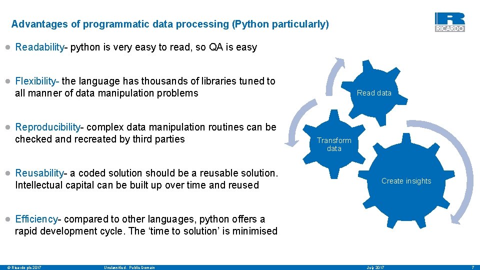
Advantages of programmatic data processing (Python particularly) • Readability- python is very easy to read, so QA is easy • Flexibility- the language has thousands of libraries tuned to all manner of data manipulation problems • Reproducibility- complex data manipulation routines can be checked and recreated by third parties • Reusability- a coded solution should be a reusable solution. Intellectual capital can be built up over time and reused Read data Transform data Create insights • Efficiency- compared to other languages, python offers a rapid development cycle. The ‘time to solution’ is minimised © Ricardo plc 2017 Unclassified - Public Domain July 2017 7

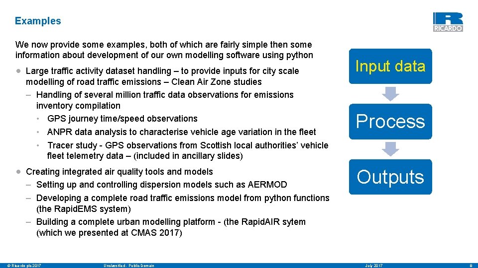
Examples We now provide some examples, both of which are fairly simple then some information about development of our own modelling software using python • Large traffic activity dataset handling – to provide inputs for city scale modelling of road traffic emissions – Clean Air Zone studies – Handling of several million traffic data observations for emissions inventory compilation • GPS journey time/speed observations • ANPR data analysis to characterise vehicle age variation in the fleet • Tracer study - GPS observations from Scottish local authorities’ vehicle fleet telemetry data – (included in ancillary slides) • Creating integrated air quality tools and models – Setting up and controlling dispersion models such as AERMOD – Developing a complete road traffic emissions model from python functions (the Rapid. EMS system) – Building a complete urban modelling platform - (the Rapid. AIR sytem (which we presented at CMAS 2017) © Ricardo plc 2017 Unclassified - Public Domain Input data Process Outputs July 2017 8

Processing traffic observations for city scale modelling © Ricardo plc 2017 Unclassified - Public Domain July 2017 9

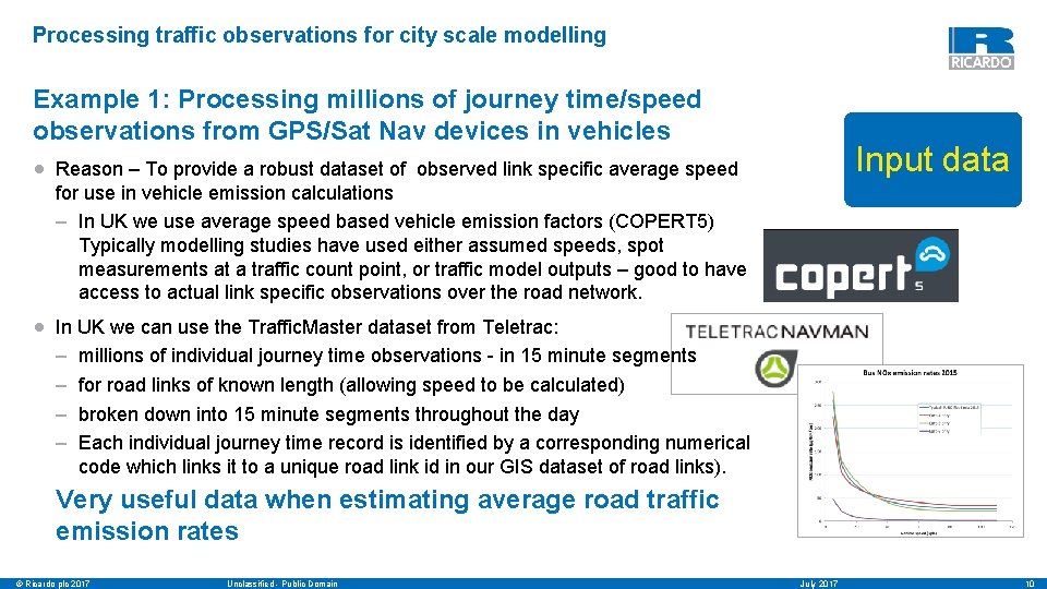
Processing traffic observations for city scale modelling Example 1: Processing millions of journey time/speed observations from GPS/Sat Nav devices in vehicles Input data • Reason – To provide a robust dataset of observed link specific average speed for use in vehicle emission calculations – In UK we use average speed based vehicle emission factors (COPERT 5) Typically modelling studies have used either assumed speeds, spot measurements at a traffic count point, or traffic model outputs – good to have access to actual link specific observations over the road network. • In UK we can use the Traffic. Master dataset from Teletrac: – millions of individual journey time observations - in 15 minute segments – for road links of known length (allowing speed to be calculated) – broken down into 15 minute segments throughout the day – Each individual journey time record is identified by a corresponding numerical code which links it to a unique road link id in our GIS dataset of road links). Very useful data when estimating average road traffic emission rates © Ricardo plc 2017 Unclassified - Public Domain July 2017 10

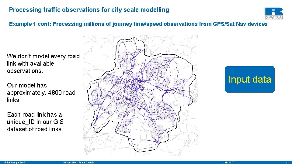
Processing traffic observations for city scale modelling Example 1 cont: Processing millions of journey time/speed observations from GPS/Sat Nav devices We don’t model every road link with available observations. Our model has approximately. 4800 road links Input data Each road link has a unique_ID in our GIS dataset of road links © Ricardo plc 2017 Unclassified - Public Domain July 2017 11

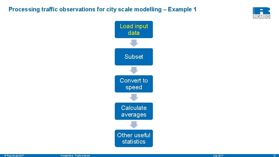
Processing traffic observations for city scale modelling – Example 1 Load input data Subset Convert to speed Calculate averages Other useful statistics © Ricardo plc 2017 Unclassified - Public Domain July 2017 12

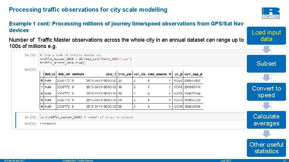
Processing traffic observations for city scale modelling Example 1 cont: Processing millions of journey time/speed observations from GPS/Sat Nav devices Number of Traffic Master observations across the whole city in an annual dataset can range up to 100 s of millions e. g. Load input data Subset Convert to speed Calculate averages Other useful statistics © Ricardo plc 2017 Unclassified - Public Domain July 2017 13

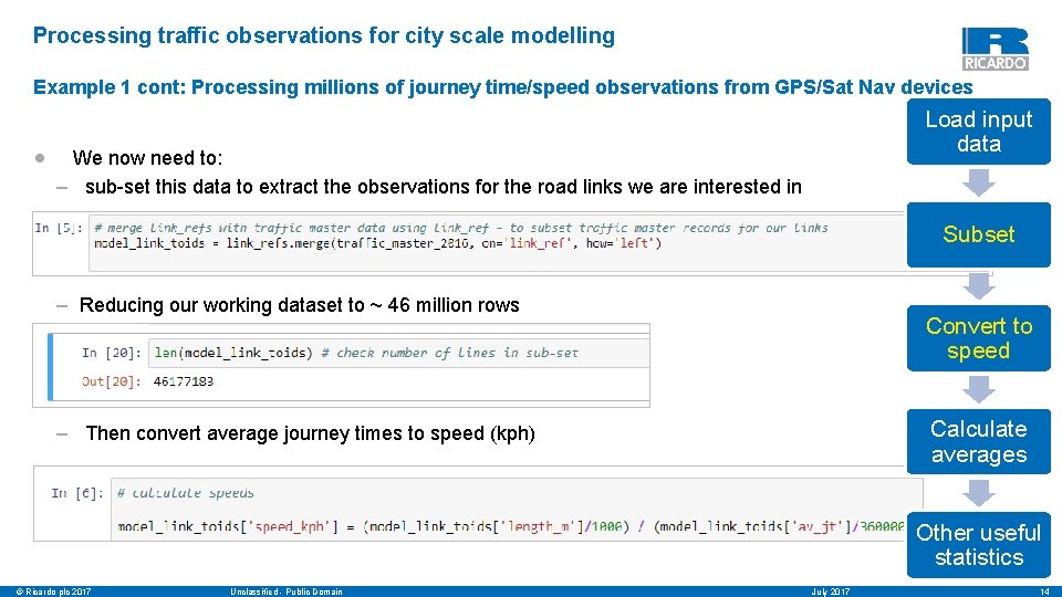
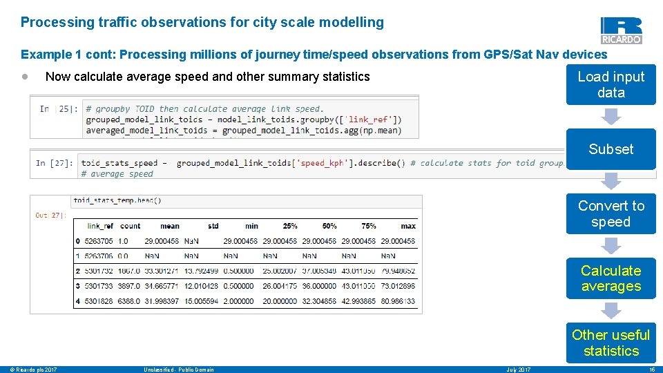
Processing traffic observations for city scale modelling Example 1 cont: Processing millions of journey time/speed observations from GPS/Sat Nav devices • Load input data We now need to: – sub-set this data to extract the observations for the road links we are interested in Subset – Reducing our working dataset to ~ 46 million rows Convert to speed Calculate averages – Then convert average journey times to speed (kph) Other useful statistics © Ricardo plc 2017 Unclassified - Public Domain July 2017 14

Processing traffic observations for city scale modelling Example 1 cont: Processing millions of journey time/speed observations from GPS/Sat Nav devices • Load input data Now calculate average speed and other summary statistics Subset Convert to speed Calculate averages Other useful statistics © Ricardo plc 2017 Unclassified - Public Domain July 2017 15

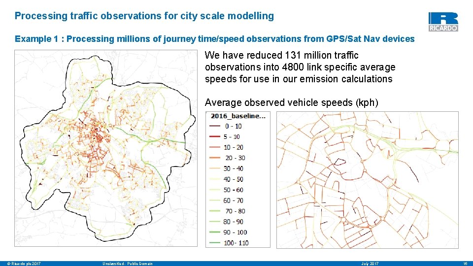
Processing traffic observations for city scale modelling Example 1 : Processing millions of journey time/speed observations from GPS/Sat Nav devices We have reduced 131 million traffic observations into 4800 link specific average speeds for use in our emission calculations Average observed vehicle speeds (kph) © Ricardo plc 2017 Unclassified - Public Domain July 2017 16

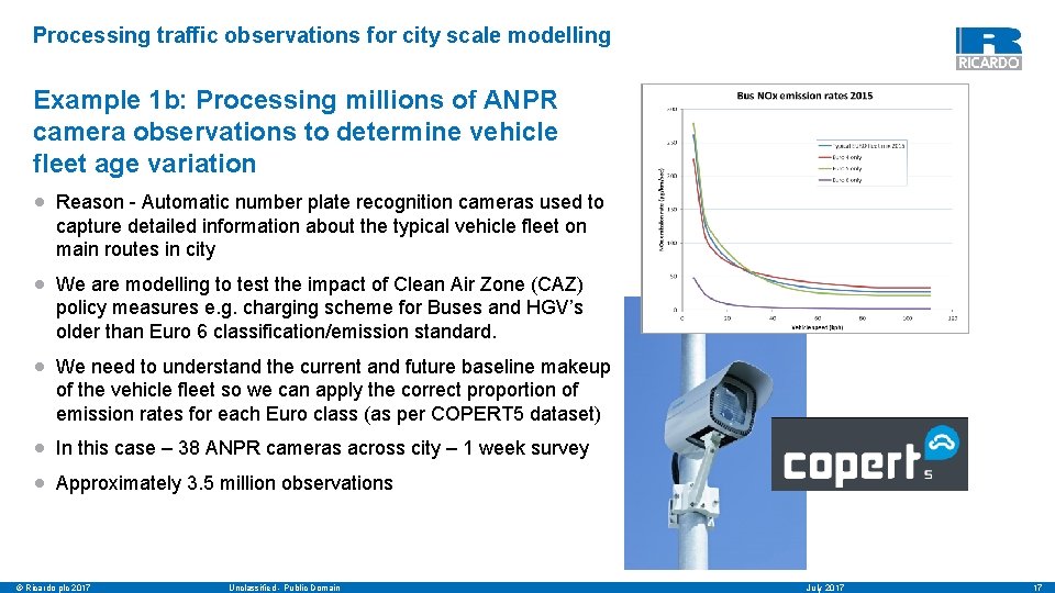
Processing traffic observations for city scale modelling Example 1 b: Processing millions of ANPR camera observations to determine vehicle fleet age variation • Reason - Automatic number plate recognition cameras used to capture detailed information about the typical vehicle fleet on main routes in city • We are modelling to test the impact of Clean Air Zone (CAZ) policy measures e. g. charging scheme for Buses and HGV’s older than Euro 6 classification/emission standard. • We need to understand the current and future baseline makeup of the vehicle fleet so we can apply the correct proportion of emission rates for each Euro class (as per COPERT 5 dataset) • In this case – 38 ANPR cameras across city – 1 week survey • Approximately 3. 5 million observations © Ricardo plc 2017 Unclassified - Public Domain July 2017 17

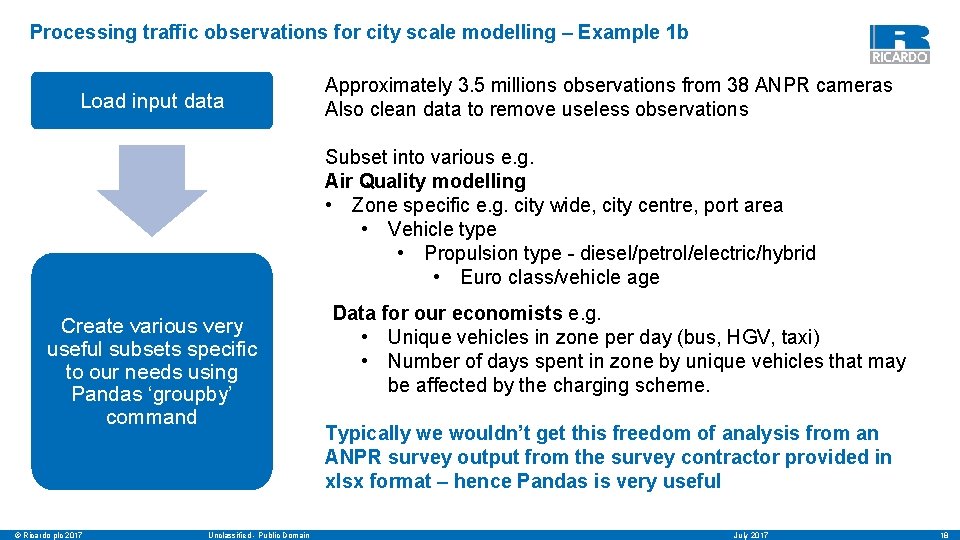
Processing traffic observations for city scale modelling – Example 1 b Load input data Approximately 3. 5 millions observations from 38 ANPR cameras Also clean data to remove useless observations Subset into various e. g. Air Quality modelling • Zone specific e. g. city wide, city centre, port area • Vehicle type • Propulsion type - diesel/petrol/electric/hybrid • Euro class/vehicle age Create various very useful subsets specific to our needs using Pandas ‘groupby’ command © Ricardo plc 2017 Unclassified - Public Domain Data for our economists e. g. • Unique vehicles in zone per day (bus, HGV, taxi) • Number of days spent in zone by unique vehicles that may be affected by the charging scheme. Typically we wouldn’t get this freedom of analysis from an ANPR survey output from the survey contractor provided in xlsx format – hence Pandas is very useful July 2017 18

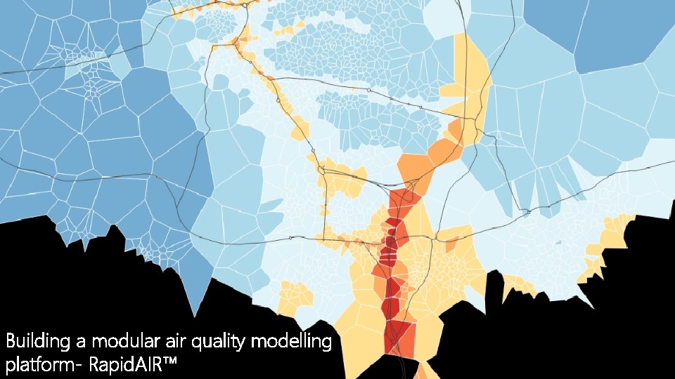
Building a modular air quality modelling platform- Rapid. AIR™ © Ricardo plc 2017 Unclassified - Public Domain July 2017 19

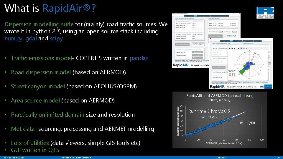
What is Rapid. Air®? Dispersion modelling suite for (mainly) road traffic sources. We wrote it in python 2. 7, using an open source stack including numpy, gdal and scipy. which automates much of the workflow for dispersion modelling for road t • Traffic emissions model- COPERT 5 written in pandas • Road dispersion model (based on AERMOD) • Street canyon model (based on AEOLIUS/OSPM) Rapid. AIR and AERMOD (annual mean, NOx, ugm 3) • Practically unlimited domain size and resolution • Met data- sourcing, processing and AERMET modelling • Lots of utilities (data viewers, simple GIS tools etc) • GUI written in QT 5 GUI) © Ricardo plc 2017 Unclassified - Public Domain rapidair (annual mean nox • Area source model (based on AERMOD) 120 Run time 5 hrs Vs 0. 5 seconds 100 80 60 R 2 = 0, 991 40 20 0 0 20 40 60 80 AERMOD (annual mean NOx) July 2017 100 120 20

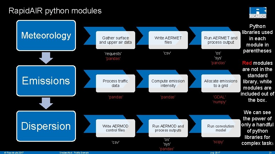
Rapid. AIR python modules Meteorology Gather surface and upper air data ‘requests’ ‘pandas’ Emissions Dispersion Unclassified - Public Domain ‘csv’ Process traffic data Compute emission intensity ‘pandas’ Write AERMOD control files ‘csv’ © Ricardo plc 2017 Write AERMET files Run AERMOD and process outputs ‘os’ ‘sys’ ‘pandas’ Run AERMET and process output ‘os’ ‘sys’ ‘pandas’ Allocate emissions to a grid ‘GDAL’ ‘numpy’ Run convolution model ‘scipy’ July 2017 Python libraries used in each module in parentheses Red modules are not in the standard library, white modules are included out of the box. We can see the power of only a handful of python libraries for complex tasks 21

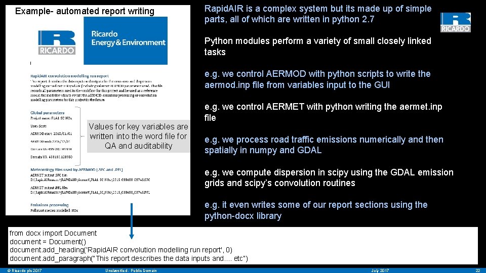
Example- automated report writing Rapid. AIR is a complex system but its made up of simple parts, all of which are written in python 2. 7 Python modules perform a variety of small closely linked tasks e. g. we control AERMOD with python scripts to write the aermod. inp file from variables input to the GUI Values for key variables are written into the word file for QA and auditability e. g. we control AERMET with python writing the aermet. inp file e. g. we process road traffic emissions numerically and then spatially in numpy and GDAL e. g. we compute dispersion in scipy using the GDAL emission grids and scipy’s convolution routines e. g. it even writes some of our report sections using the python-docx library from docx import Document document = Document() document. add_heading(‘Rapid. AIR convolution modelling run report', 0) document. add_paragraph(“This report describes the data inputs and. . etc”) © Ricardo plc 2017 Unclassified - Public Domain July 2017 22

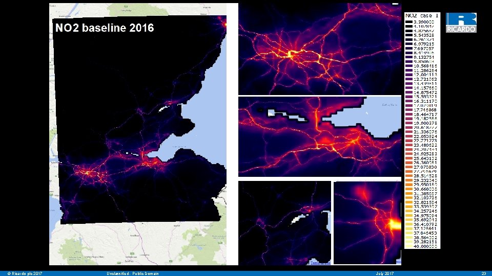
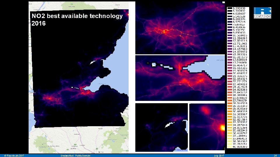
© Ricardo plc 2017 Unclassified - Public Domain July 2017 23

NO 2 in 2016 – the baseline © Ricardo plc 2017 Unclassified - Public Domain July 2017 24

Ancillary material © Ricardo plc 2017 Unclassified - Public Domain July 2017 25

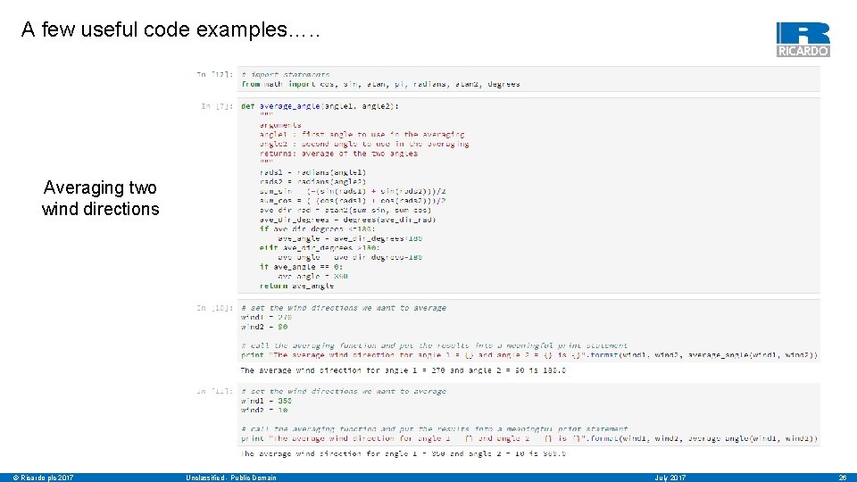
A few useful code examples…. . Averaging two wind directions © Ricardo plc 2017 Unclassified - Public Domain July 2017 26

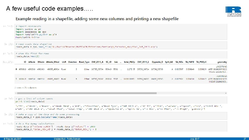
A few useful code examples…. . © Ricardo plc 2017 Unclassified - Public Domain July 2017 27

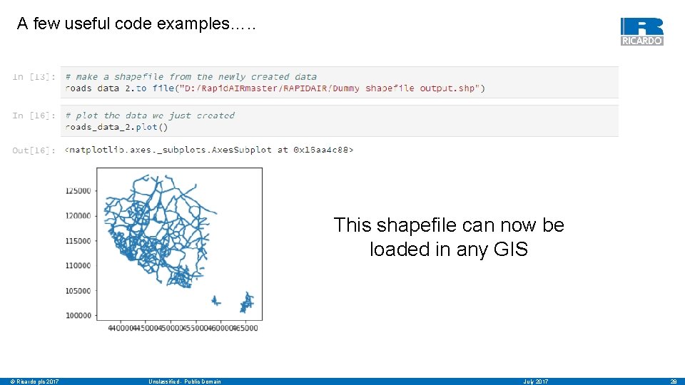
A few useful code examples…. . This shapefile can now be loaded in any GIS © Ricardo plc 2017 Unclassified - Public Domain July 2017 28

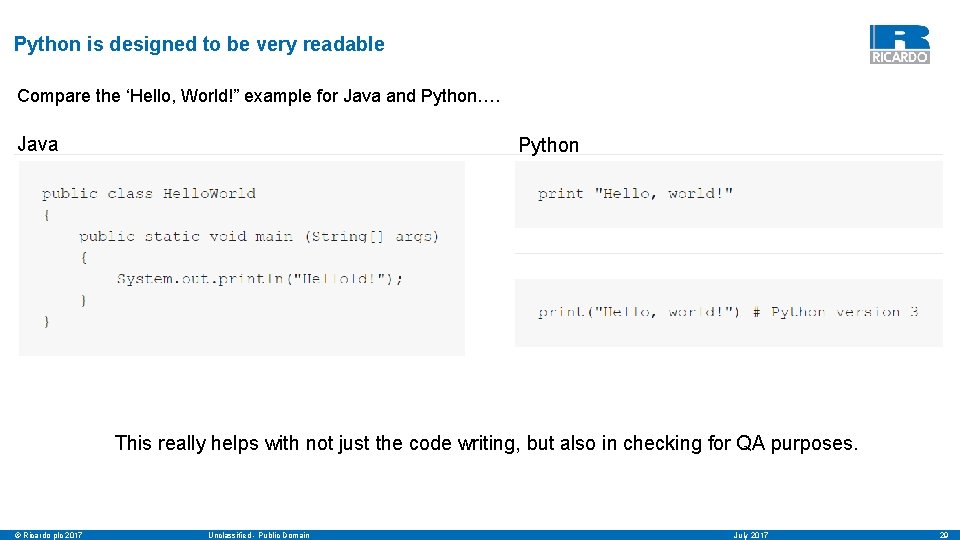
Python is designed to be very readable Compare the ‘Hello, World!” example for Java and Python…. Java Python This really helps with not just the code writing, but also in checking for QA purposes. © Ricardo plc 2017 Unclassified - Public Domain July 2017 29

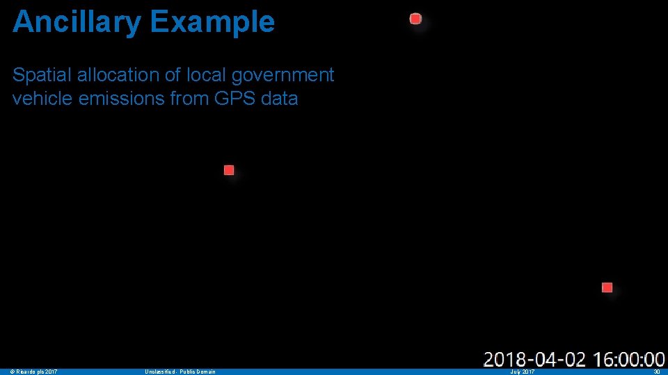
Ancillary Example Spatial allocation of local government vehicle emissions from GPS data © Ricardo plc 2017 Unclassified - Public Domain July 2017 30

Problem statement Diagnose the source emission signal from local government vehicles transiting small towns during business hours Key things we need: 1) Processing of GPS measurements 2) Computation of emissions for each time step and vehicle 3) Spatial allocation of emissions to help inventory compilation 4) More modular approach with scripts ‘talking’ to each other Python’s flexibility allows all of this using only a few libraries The project allowed us to add significant value to an existing dataset (GPS) © Ricardo plc 2017 Unclassified - Public Domain July 2017 31

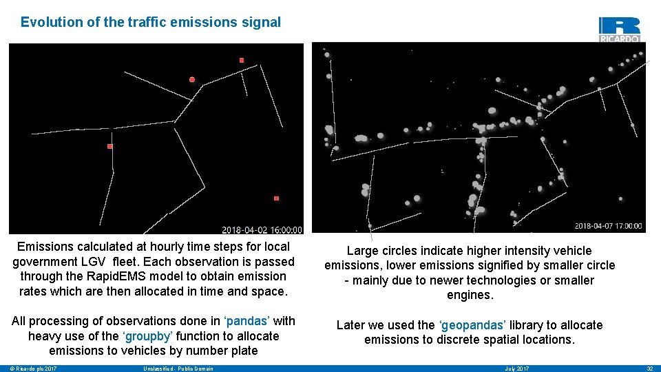
Evolution of the traffic emissions signal Emissions calculated at hourly time steps for local government LGV fleet. Each observation is passed through the Rapid. EMS model to obtain emission rates which are then allocated in time and space. Large circles indicate higher intensity vehicle emissions, lower emissions signified by smaller circle - mainly due to newer technologies or smaller engines. All processing of observations done in ‘pandas’ with heavy use of the ‘groupby’ function to allocate emissions to vehicles by number plate Later we used the ‘geopandas’ library to allocate emissions to discrete spatial locations. © Ricardo plc 2017 Unclassified - Public Domain July 2017 32