Pulse Thunderstorm Operating Strategies Mike Cammarata NOAANWS Columbia

Pulse Thunderstorm Operating Strategies Mike Cammarata NOAA/NWS Columbia, SC

Overview § § Introduction What we look at What we look for An example
 – May – June – July")
Climatology § Thunderstorm days at CAE (per LCD) – May – June – July – August 6. 1 9. 3 12. 3 9. 4 § That’s at a point…we have radar ops for predominately pulse storms on the order of twice those numbers § Prime time … noon through 8 pm

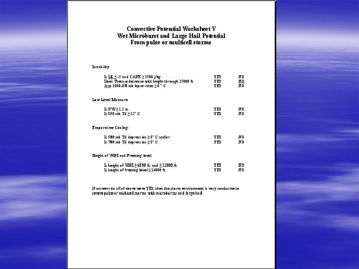
Pulse Storm Severe Weather Threat § Microbursts – Less than 4 km in outflow diameter – Peak winds last 2 -5 min at most – Potential for F 0 – F 1 wind damage – Wind shear may reduce aircraft performance § Large Hail – Usually 0. 75 to 1. 00 in

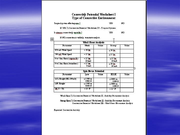
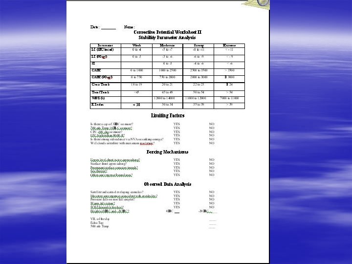
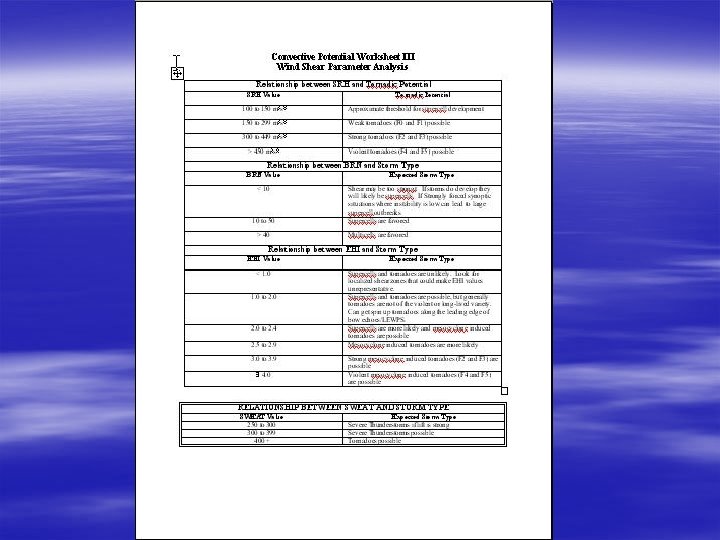
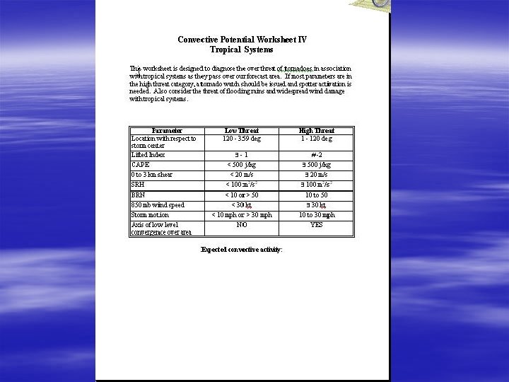
Convective Potential Analysis § Analysis of stability and shear paramteters § During the convective season we do this every day at least twice per day § Important to anticipate convective mode and type of threat § Factors into warning decision e. g. , if downburst threat is high, more likely to issue warning for marginal criteria

Mesoscale Desk § Ongoing meso analysis helps us to anticipate convective initiation and monitor Near Storm Environment for ongoing event § Satellite and lightning data very important § Look for trends § Satellite sounder data § ACARS data

Mesoscale Desk http: //www. orbit. nesdis. noaa. gov/smcd/opdb/aviation/mb. html

Mesoscale Desk § http: //www. orbit. nesdis. noaa. gov/smcd/opdb/aviation/mb. html – – – – LI TPW CAPE CIN WINDEX Theta-e deficit SFC – 300 mb Wet Microburst Severity Index (WMSI) GOES Soundings

Mesoscale Desk http: //www. orbit. nesdis. noaa. gov/smcd/opdb/aviation/mb. html
 integrates data from virtually")
Mesoscale Desk § The Local Analysis and Prediction System (LAPS) integrates data from virtually every meteorological observation system into a very high -resolution gridded framework centered on a forecast office's domain of responsibility. Thus, the data from local mesonetworks of surface observing systems, Doppler radars, satellites, wind and temperature (RASS) profilers (404 and boundary-layer 915 MHz), radiometric profilers, as well as aircraft are incorporated every hour into a three-dimensional grid covering a 1040 km by 1240 km area.

Mesoscale Desk § LAPS Sounding for CAE

Mesoscale Desk § LAPS CAPE § LAPS SFC Wind § Radar mosaic § LAPS analyses are available for a variety of surface and upper air fields

Mesoscale Desk SPC Web site – Composite Maps and Hourly Mesoscale Analyses http: //www. spc. noaa. gov/exper/mesoanalysis/s 1/index 2. html

Staffing § Minimum requirements – Radar operator/Warning Met – Meso (TAF’s, NOW, SPS, ongoing convective and meso analysis) – Synoptic (grids, updates to public products) – HMT (2) (NWR, NOW, SPS, LSR, Hydro) – Coordinator – Ham Radio Net Controller(s) – Additional staff if widespread convection – Sectorize if you can – Polygon beta test site § Verification … real time and subsequent day

What we look at § CR/VIL Combo – Lower values filtered (<30 d. Bz, <30 g/kg) – Highlights stronger cells, cuts down on clutter – Looping reveals trends – Filtering can highlight outflows § Overlay – Lightning (look for trends) – MSAS wind barbs (convergence) – LAPS/MSAS LI or Cape (instability)

What we look at § CR § Laps wind barbs § Lightning

What we look at § Good example of color scheme highlighting outflow boundaries
, LRM 3 (>34 kft),")
What we look at § LRM 2 (24 -34 kft), LRM 3 (>34 kft), ULR, VIL, ET – Lower values filtered – Look for values surpassing thresholds – ULR can be set based on expected height of storm or temp level e. g. , -20 C

What we look at § 4 Panel – – § § VIL CR LRM 2 LRM 3 63 d. BZ > 24 k ft 56 d. BZ > 33 k ft

What we look at § All tilts Z/V 8 bit – monitor data as it arrives – Elevated high reflectivity cores – MARC signatures – Storm top divergence – Strong low level winds § 4 -panel Displays can be used as well

What we look at § 4 Panel display shows high reflectivity cores and TBSS
 – High reflectivity cores – Tilt")
What we look at § RCS (used heavily) – High reflectivity cores – Tilt § VCS (used by some) – Storm Top Divergence – Mid-level convergence – Near ground divergence – outflow

Supercell Storm!

What we look at § CR/VIL, LRM’s, ET’s from adjacent offices – Different perspective – Corroboration – Cone of silence

What we look at § Base Velocity 0. 5 8 bit – Look for strong low level radial velocities – use a “compressed” 8 bit color curve to better highlight velocities near threshold values. – Only good within 30 nm of radar – By the time a downburst signature shows up in the data it may be too late for lead time

What we look at § Base Velocity image showing thunderstorm downburst signature

What we look at § Scan – Trend Set – VIL, d. BZ ht, top, posh – Good for prioritizing and assessing trends with individual cells – Filter based on VIL or dbz

What we look at

What we look at § Satellite and observed data – IR and VIS – Surface obs including mesonet data – MSAS and LAPS § LI CAPE § Pressure change § Wind barbs
 Mesonet sites (blue)")
What we look at § § ASOS sites (yellow) Mesonet sites (blue)

What we look for § VIL decreases by at least 10 kg/m 2 and § Height of max reflectivity decreases by at least 8 kft. (Storm collapse) § POD. 88 and FAR. 25 – Reference … An Overview of Operational Forecasting for Wet Microbursts. William P. Roeder 45 th Weather Squadron, USAF – http: //www. wdtb. noaa. gov/workshop/psdp/ – WDTB Pulse Storm Downburst Prediction Workshop § Use VIL … SCAN § May be too late for lead time by the time the storm collapses

What we look for See 02 Aug 2002 WES Sim guide § Relatively higher height of first echo appearance (20 -30 kft) for severe storms vs. non-severe (10 -20 kft) § Usually maintain 50 -55 d. BZ closed reflectivity contour as core descends § Centroid of high reflectivity core above 25 kft and top of core above 30 kft § Old rule 55 d. BZ above 30 kft § Use RCS and/or All tilts Z/V 8 bit

What we look for See 02 Aug 2003 WES Sim guide § MARC signature – 50 kt convergence in 5 -11 kft AGL layer – Convergence in or near high reflectivity core – Works up to 90 miles from radar (Falk et al. 1998) § Use All tilts Z/V 8 bit, VCS

What we look for MARC signature http: //www. srh. noaa. gov/shv/Downburst_Climo. htm

What we look for Reference Mackey 1998 http: //www. wdtb. noaa. gov/workshop/psdp/index. htm

What we look for Reference Mackey 1998 http: //www. wdtb. noaa. gov/workshop/psdp/index. htm

What we look for TBSS

What we look for TBSS

What we look for § 4 Panel display showing monster TBSS and high reflectivity core § This storm produced baseball size hail

What we look for CAE VIL of the Day § Computed as part of Convective potential analysis § Logistic Regression equation …predictand is the probability of large hail § Predictors include VIL, VIL density, 500 mb T, and Totals index

What we look for CAE VIL of the Day
 / ET (kft) §")
What we look for § VIL Density = VIL (g/kg) / ET (kft) § Values > 3. 5 had a. 9 POD at TUL – Amburn, S. A. and P. L. Wolf, 1997: VIL density as a hail indicator. Wea. and Forecasting, 12, 473 -478. – Greg Tipton, John Di. Stefano WFO Wilmington, Ohio § Use 4 panel VIL ET LRM 2 LRM 3

What we look for From OTB now WDTB § Storm Top Divergence – >. 75 in – 1. 75 in – 2. 50 in – 2. 75 in – 4. 00+ in |Vout| + |Vin| 80 – 110 kt 110 – 135 kt 135 – 175 kt 175 – 225 kt > 225 kt § Use All tilts Z/V 8 bit, VCS

What we look for § Height of 65 d. BZ § 96% severe if above freezing level – Gerard, A. , 1998: Operational observations of Extreme Reflectivity values in Convective Cells. Natl. Wea. Digest, 22, 3 -8. – Greg Tipton, John Di. Stefano WFO Wilmington, Ohio § Very soon after getting 88 D in 1994 we noticed this to be highly reliable indicator § Good for severe hail and/or wind § Use RCS and/or All tilts Z/V 8 bit

Verification § Sources – – – County EM Directors County EM Dispatch Local Sheriff, Police, Fire depts. Spotters HAM net Post Offices Local and regional Utilities State and local parks and marinas Media Churches Phone book and Street Atlas

An Example – 17 May 2005 § § § Weakly sheared environment Weak to moderate instability Cold pool aloft with upper low over area WBZ 9400 ft Freezing level around 12000 ft VIL of Day 43 g/kg

An Example – 17 May 2005 § § Reflectivity 1905 GMT Core - 17200 ft 43 d. BZ

An Example – 17 May 2005 § § § Reflectivity 1911 GMT Core 18500 ft 67 d. BZ TBSS WBZ 9400 ft

An Example – 17 May 2005 § § § Reflectivity 1915 GMT Core 19600 ft 68 d. BZ TBSS

An Example – 17 May 2005 § LRM 2 24 -33 k ft § 1905 GMT § Nothing

An Example – 17 May 2005 § § LRM 2 24 -33 k ft 1915 GMT 50 -57 d. BZ Significant increase in 10 min

An Example – 17 May 2005 § RCS § 1915 GMT § 65 -70 d. BZ elevated core to around 15 k ft

An Example – 17 May 2005 § § KCLX VIL 1905 GMT 10 -15 g/kg KCAE VIL never got above 35 g/kg … close to radar

An Example – 17 May 2005 § § § KCLX VIL 1910 GMT 5 -10 g/kg

An Example – 17 May 2005 § § § KCLX VIL 1915 GMT 25 -30 g/kg

An Example – 17 May 2005 § § KCLX VIL 1920 GMT 45 -50 g/kg VIL of day was 43 g/kg § Note that VIL reached highest value about 10 mins after other products

An Example – 17 May 2005 § Warning was issued based on TBSS from 1911 GMT scan § At 1930 received several reports of. 88 in hail
- Slides: 62