Pulse And Digital Modulation Techniques UNIT III Pulse

Pulse And Digital Modulation Techniques UNIT III

Pulse And Digital Modulation Techniques Pulse Modulation Techniques: Pulse Analog Modulation Techniques, sampling, Pulse Digital Modulation Techniques: PCM, DPCM, Average Information, Entropy, Information Rate. Source coding: Shanon-Fano, Huffman and Limpel-Ziv Digital-to-digital Conversion: Line Coding, Line Coding Schemes, Block Coding, Scrambling Digital-to-analog Conversion: Aspects of Digital-to-Analog Conversion, Amplitude Shift Keying (ASK), Frequency Shift Keying (FSK), Phase Shift Keying (PSK), Quadrature Amplitude Modulation (QAM) Analog-to-analog Conversion: Amplitude Modulation,

Pulse Modulation Pulse modulation is the process of changing a binary pulse signal to represent the information to be transmitted. The primary benefits of transmitting information by binary techniques arise from the great noise tolerance and the ability to regenerate the degraded signal. It is the process of transmitting signals in the form of pulses (discontinuous signals) by using special technique. It consists of sampling analog information signal, then converting those samples to discrete pulses and transporting the pulses from a source to a destination over a physical transmission medium.

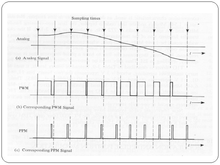
Pulse Analog Modulation In analog pulse modulation, a periodic pulse train is used as the carrier wave, and some characteristic feature of each pulse (e. g. , amplitude, duration, or position) is varied in a continuous manner in accordance with the corresponding sample value of the message signal. Thus, in analog pulse modulation, information is transmitted basically in analog form, but the transmission takes place at discrete times. Types are: PAM, PDM, PPM

Pulse Digital Modulation In digital pulse modulation, on the other hand, the message signal is represented in a form that is discrete in both time and amplitude, thereby permitting its transmission in digital form as a sequence of coded pulses.

Types of Pulse Analog Modulation Pulse Width Modulation (PWM) / Pulse Duration Modulation (PDM) Pulse Position Modulation (PPM) Pulse Amplitude Modulation (PAM)

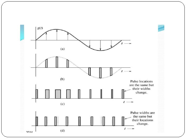
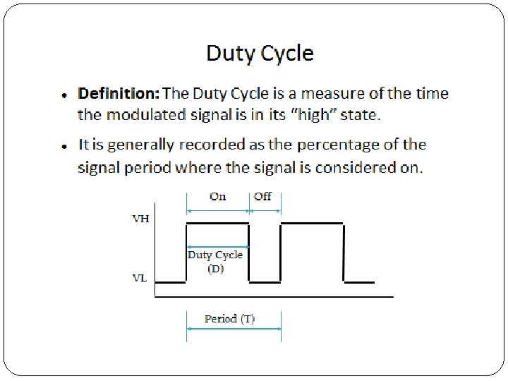
1. Pulse Width Modulation (PWM) / Pulse Duration Modulation (PDM) It is a modulation technique used to encode a message into a pulsing signal. Although this modulation technique can be used to encode information for transmission, its main use is to allow the control of the power supplied to electrical devices. The longer the switch is on compared to the off periods, the higher the total power supplied to the load. The on-off behavior changes the average power of signal. Output signal alternates between on and off within a specified period. If signal toggles between on and off quicker than

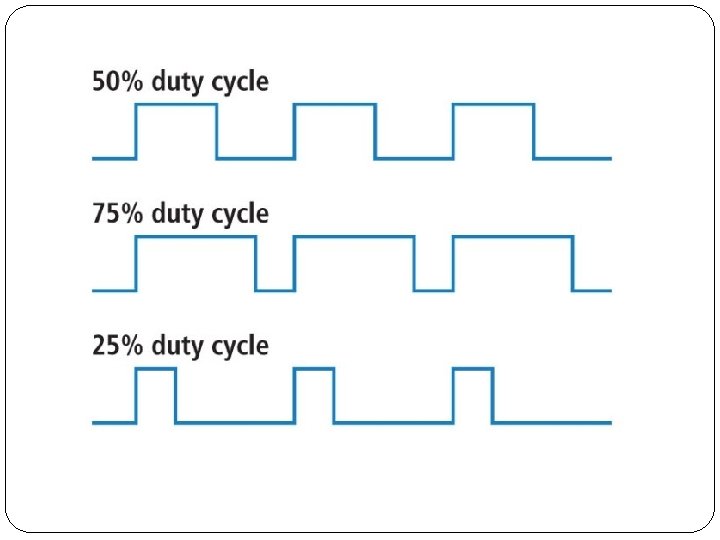
Duty cycle is expressed in percent, 100% being fully on.

The main advantage of PWM is that power loss in the switching devices is very low. When a switch is off there is practically no current, and when it is on and power is being transferred to the load, there is almost no voltage drop across the switch. Power loss, being the product of voltage and current, is thus in both cases close to zero. PWM also works well with digital controls, which, because of their on/off nature, can easily set the needed duty cycle.

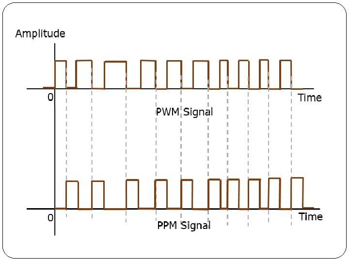
2. Pulse Position Modulation (PPM) In PPM, data are transmitted with short pulses. All pulses have both the same width and amplitude. The parameter that changes is the delay between each pulse. In PPM the amplitude and width of the pulses is kept constant but the position of each pulse is varied accordance with the amplitudes of the sampled value of the modulating signal. The position of the pulses is changed with respect to the position of reference pulses. The PPM pulses can be derived from the PWM pulses.

With the increase in the modulating voltage the PPM pulse shift further with respect to reference. The vertical dotted lines drawn in Fig are treated as reference lines to measure the shift in position of PPM pulses. Each trailing of the pulse width modulated signal becomes the starting point for pulses in PPM signal. Hence, the position of these pulses is proportional to the width of the PWM pulses.

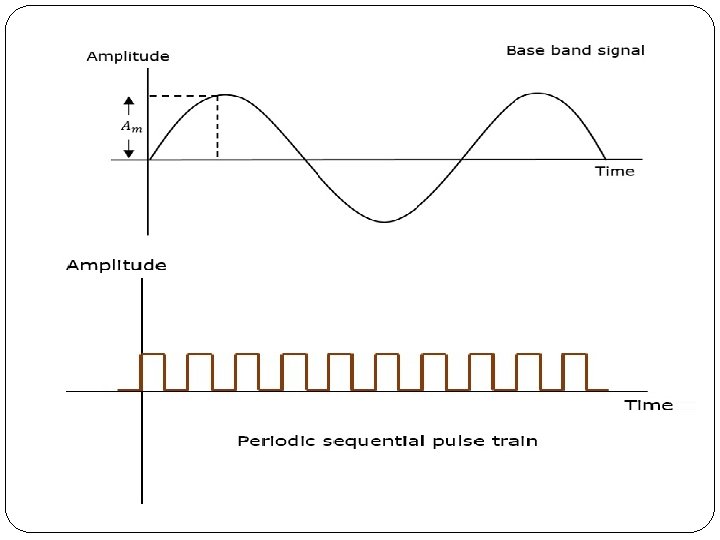
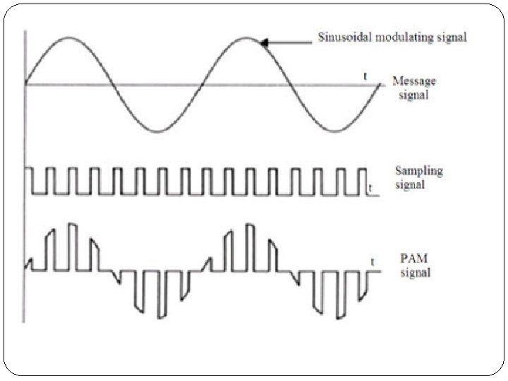
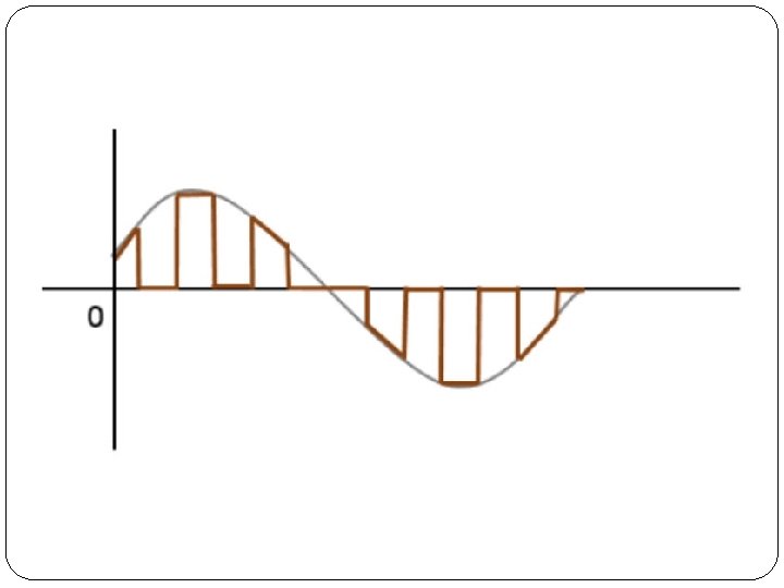
3. Pulse Amplitude Modulation (PAM) Pulse amplitude modulation is the basic form of pulse modulation. In this modulation, the signal is sampled at regular intervals and each sample is made proportional to the amplitude of the modulating signal. Pulse amplitude modulation is a technique in which the amplitude of each pulse is controlled by the instantaneous amplitude of the modulation signal. It is a modulation system in which the signal is sampled at regular intervals and each sample is made proportional to the amplitude of the signal at the instant of sampling.

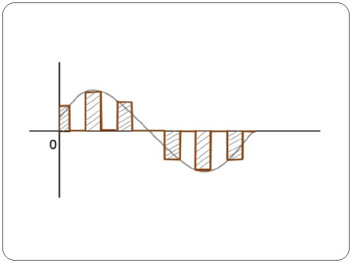
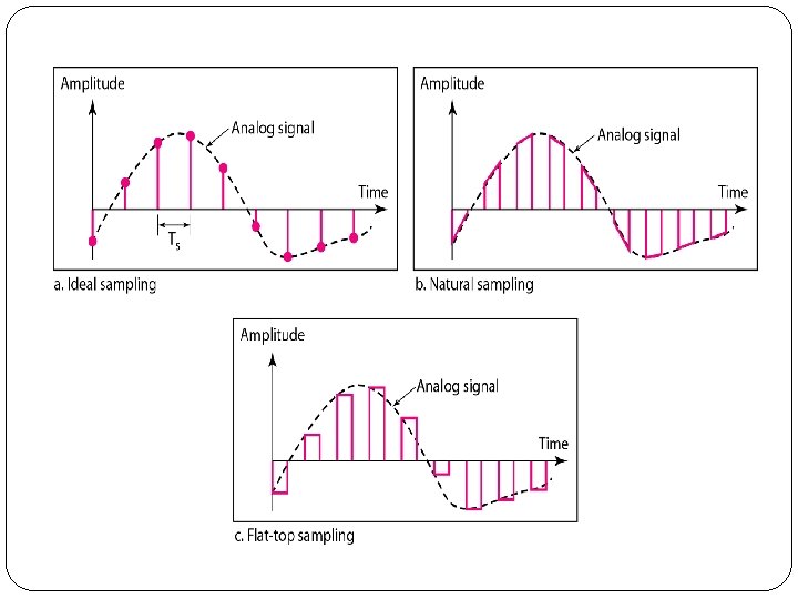
There are two types of sampling techniques for transmitting a signal using PAM. They are: Flat Top PAM Natural PAM Flat Top PAM: The amplitude of each pulse is directly proportional to modulating signal amplitude at the time of pulse occurrence. The amplitude of the signal cannot be changed with respect to the analog signal to be sampled. The tops of the amplitude remain flat.

Natural PAM: The amplitude of each pulse is directly proportional to modulating signal amplitude at the time of pulse occurrence. Then follows the amplitude of the pulse for the rest of the half cycle.

PAM Amplitude is varied PWM Width is varied PPM Position is varied Bandwidth depends on the width of the pulse rise time of the pulse Instantaneous transmitter power varies with the amplitude of the pulses Instantaneous transmitter power varies with the amplitude and width of the pulses Instantaneous transmitter power remains constant with the width of the pulses System complexity is high System complexity is low Noise interference is high Noise interference is low It is similar to amplitude modulation It is similar to frequency modulation It is similar to phase modulation

Types of Pulse Digital Modulation Pulse Code Modulation (PCM) Delta Modulation (DM) Differential Pulse-Code Modulation (DPCM)

1. Pulse Code Modulation (PCM) Pulse code modulation is a method that is used to convert an analog signal into a digital signal, so that it can be transmitted through the digital communication network. Instead of a pulse train, PCM produces a series of numbers or digits, and hence this process is called as digital. We can also get back our analog signal by demodulation.

Each one of these digits, though in binary code, represent the approximate amplitude of the signal sample at that instant. In Pulse Code Modulation, the message signal is represented by a sequence of coded pulses. This message signal is achieved by representing the signal in discrete form in both time and amplitude.

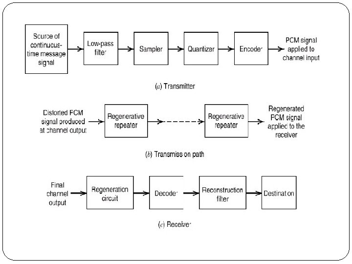
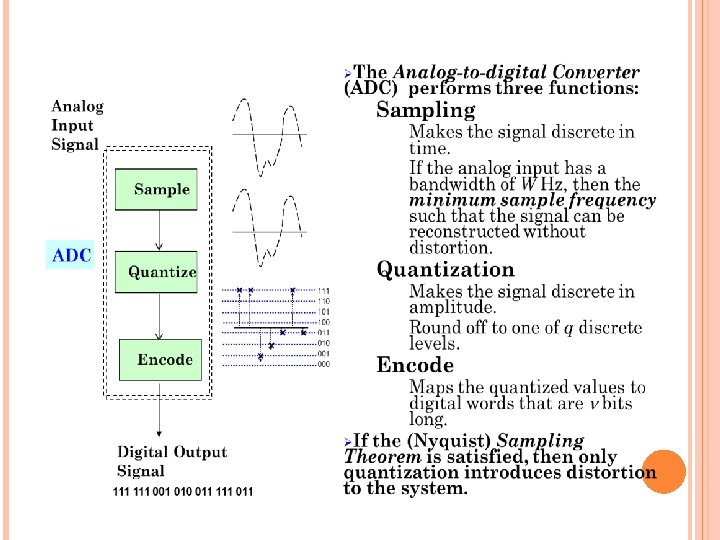
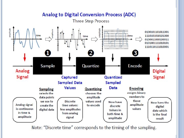
Basic Elements of PCM The Pulse Code Modulation process is done in three steps Sampling, Quantization, and Coding. Sampling operation generates a flat-top PAM signal. Quantizing operation approximates the analog values by using a finite number of levels. This operation is considered in 3 steps Uniform Quantizer Quantization Error Quantized PAM signal output PCM signal is obtained from the quantized PAM signal by encoding each quantized sample value into a digital word.

Low Pass Filter This filter eliminates the high frequency components present in the input analog signal which is greater than the highest frequency of the message signal, to avoid aliasing of the message signal. Aliasing refers to the effect produced when a signal is imperfectly reconstructed from the original signal.

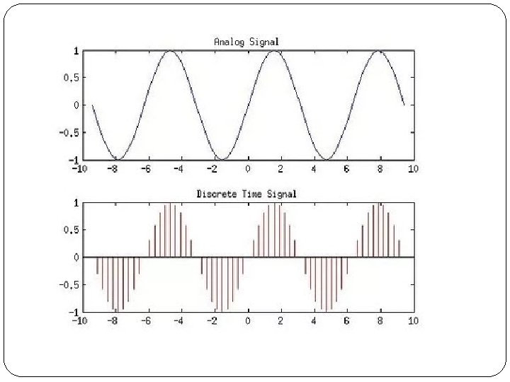
Sampler This is the technique which helps to collect the sample data at instantaneous values of message signal, so as to reconstruct the original signal. Sampling is a process of measuring the amplitude of a continuous-time signal at discrete instants, converts the continuous signal into a discrete signal. The Sample is a value or set of values at a point in time. Sampler extract samples of a continuous signal, it is a subsystem ideal sampler produces samples which are equivalent to the instantaneous value of the continuous signal at the specified various points. The Sampling process generates flat- top Pulse Amplitude Modulated (PAM) signal.

Aliasing occurs when a signal is not sampled at a high enough frequency to create an accurate representation. This effect is shown in the following example of a sinusoidal function: In this example, the dots represent the sampled data and the curve represents the original signal. Because there are too few sampled data points, the resulting pattern produced by the sampled data is a poor

Sampling frequency, Fs is the number of average samples per second also known as Sampling rate. According to the Nyquist Theorem sampling rate should be at least 2 times the upper cutoff frequency. Sampling frequency, Fs>=2*fmax to avoid Aliasing Effect. If the sampling frequency is very higher than the Nyquist rate it become Oversampling, theoretically a bandwidth limited signal can be reconstructed if sampled at above the Nyquist rate. If the sampling frequency is less than the Nyquist rate it will become Undersampling. Basically two types of techniques are used for the

Quantizer Quantizing is a process of reducing the excessive bits and confining the data. The sampled output when given to Quantizer, reduces the redundant bits and compresses the value. Encoder The digitization of analog signal is done by the encoder. It designates each quantized level by a binary code. The sampling done here is the sample-and-hold process. These three sections (LPF, Sampler, and Quantizer) will act as an analog to digital converter. Encoding minimizes the bandwidth used. Regenerative Repeater This section increases the signal strength.

QUANTIZATION EXAMPLE Analogue signal Sampling TIMING Quantization levels. Quantized to 5 -levels Quantization levels Quantized 10 -levels

Encoding The output of the quantizer is one of M possible signal levels. If we want to use a binary transmission system, then we need to map each quantized sample into an n bit binary word. Encoding is the process of representing each quantized sample by an bit code word. The mapping is one-to-one so there is no distortion introduced by encoding. Some mappings are better than others. A Gray code gives the best end-to-end performance. The weakness of Gray codes is poor performance

Decoder The decoder circuit decodes the pulse coded waveform to reproduce the original signal. This circuit acts as the demodulator. Reconstruction Filter After the digital-to-analog conversion is done by the regenerative circuit and the decoder, a low-pass filter is employed, called as the reconstruction filter to get back the original signal. Hence, the Pulse Code Modulator circuit digitizes the given analog signal, codes it and samples it, and then transmits it in an analog form. This whole process is repeated in a reverse pattern to obtain the original signal.

2. Delta Modulation In PCM the signaling rate and transmission channel bandwidth are quite large since it transmits all the bits which are used to code a sample. To overcome this problem, Delta modulation is used.

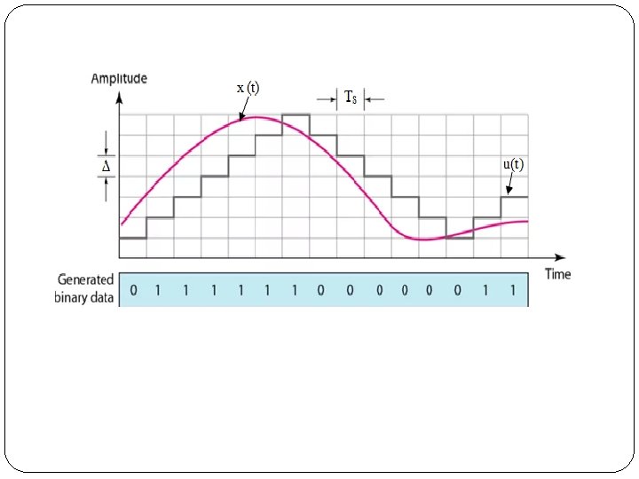
The difference between the input signal x(t) and staircase approximated signal is confined to two levels, i. e. , +Δ and -Δ. Now, if the difference is positive, then approximated signal is increased by one step, i. e. , ‘Δ’. If the difference is negative, then approximated signal is reduced by ‘Δ’. When the step is reduced, ‘ 0’ is transmitted and if the step is increased, ‘ 1’ is transmitted. Hence, for each sample, only one binary bit is

If a signal is large then, next bit in the digital data is 1, otherwise it is 0

Advantages of Delta Modulation Ø Since, the delta modulation transmits only one bit for one sample, therefore the signaling rate and transmission channel bandwidth is quite small for delta modulation compared to PCM. Ø The transmitter and receiver implementation is very much simple for delta modulation. There is no analog to digital converter required in delta modulation.

Disadvantages of Delta Modulation The delta modulation has two major drawbacks as under : Ø Slope overload distortion The rate of rise of input signal x(t) is so high that the staircase signal can not approximate it, the step size ‘Δ’ becomes too small for staircase signal u(t) to follow the step segment of x(t). This error or noise is known as slope overload distortion.

Granular or idle noise Ø Granular or Idle noise occurs when the step size is too large compared to small variation in the input signal. Ø This means that for very small variations in the input signal, the staircase signal is changed by large amount (Δ) because of large step size.

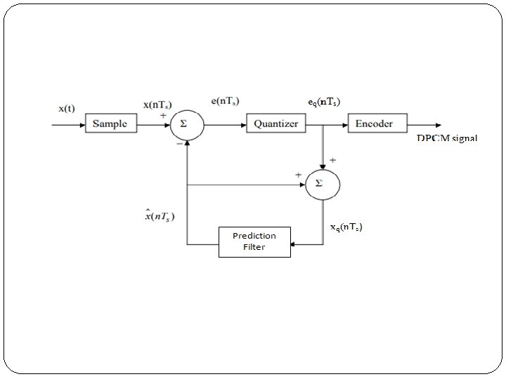
2. Differential Pulse-Code Modulation (DPCM) For the samples that are highly correlated, when encoded by PCM technique. To process this redundant information and to have a better output, it is a wise decision to take a predicted sampled value, assumed from its previous output and summarize them with the quantized values. Such a process is called as Differential PCM (DPCM) technique. DPCM is a signal encoder that uses the baseline of pulse -code modulation (PCM) but adds some functionalities based on the prediction of the samples of the signal. It is a procedure of converting an analog into a digital signal in which an analog signal is sampled and then the difference between the actual sample value and its predicted value (predicted value is based on previous

information with a little difference. Ø If this redundancy is reduced, then overall bit rate will decrease and number of bits required to transmit one sample will also be reduced. Ø We can observe from fig. 1 that the samples taken at 4 Ts , 5 Ts and 6 Ts are encoded to same value of (110).

Redundant Information in PCM

When highly correlated samples are encoded the resulting encoded signal contains redundant information. By removing this redundancy before encoding an efficient coded signal can be obtained. One of such scheme is the DPCM technique. By knowing the past behavior of a signal up to a certain point in time, it is possible to make some inference about the future values.

Advantages of DPCM Ø As the difference between x(n. Ts) and xˆ(n. Ts) is being encoded and transmitted by the DPCM technique, a small difference voltage is to be quantized and encoded. Ø This will require less number of quantization levels and hence less number of bits to represent them. Ø Thus signaling rate and bandwidth of a DPCM system will be less than that of PCM.

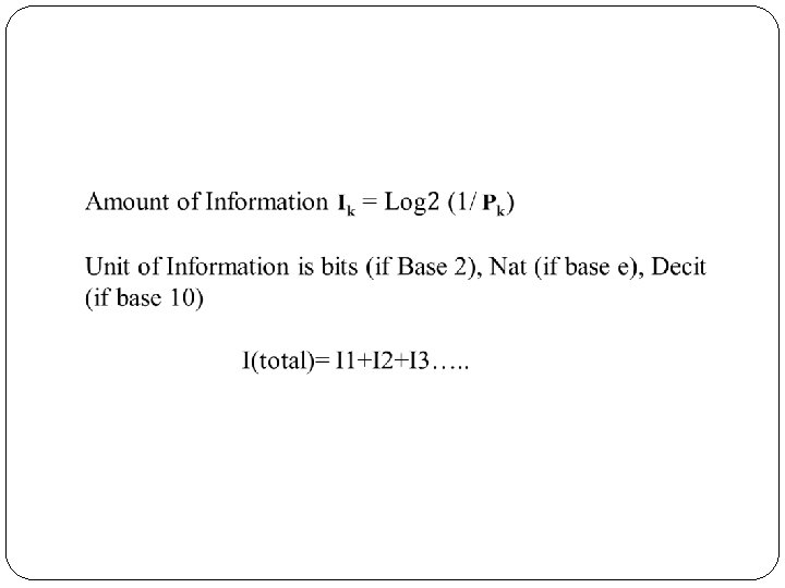
Information Theory Information is the source of a communication system, whether it is analog or digital. Information theory is a mathematical approach to the study of coding of information along with the quantification, storage, and communication of information. Conditions of Occurrence of Events If we consider an event, there are three conditions of occurrence. If the event has not occurred, there is a condition of uncertainty. If the event has just occurred, there is a condition of surprise. If the event has occurred, a time back, there is a condition of having some information.

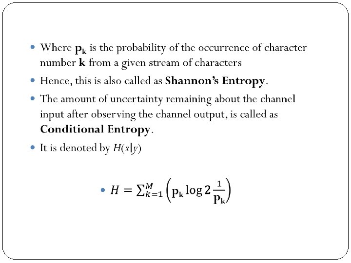
Entropy is the measure of the average information content missing from a set of data when the value of the random variable is not known. Helps determine the average number of bits needed for storage or communication of a signal. As the number of possible outcomes for a random variable increases, entropy increases. As entropy increases, information decreases. https: //www. youtube. com/watch? v=9 r 7 FIXEAGvs

The entropy, in this context, is the expected number of bits of information contained in each message, taken over all possibilities for the transmitted message. For example, suppose the transmitter wanted to inform the receiver of the result of a 4 -person tournament, where some of the players are better than others. The entropy of this message would be a weighted average of the amount of information each of the possible messages (i. e. "player 1 won", "player 2 won", "player 3 won", or "player 4 won") provides. In essence, the "entropy" can be viewed as how much useful information a message is expected to contain. It also provides a lower bound for the "size" of an encoding scheme, in the sense that the expected number of bits to be transmitted under some encoding scheme is at least the entropy of the message.

Information rate is the average entropy per symbol. R= r*H Where r= No. of messages per second H= Average information/message R= Information rate

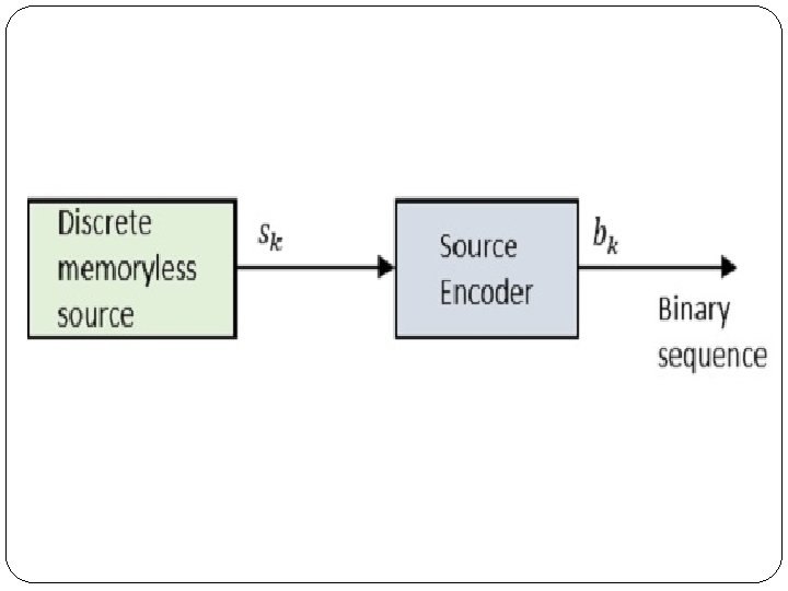
Discrete Memoryless Source A source from which the data is being emitted at successive intervals, which is independent of previous values, can be termed as discrete memoryless source. This source is discrete as it is not considered for a continuous time interval, but at discrete time intervals. This source is memoryless as it is fresh at each instant of time, without considering the previous values.

Source Coding The Code produced by a discrete memoryless source, has to be efficiently represented, which is an important problem in communications. For this to happen, there are code words, which represent these source codes.

Where Sk is the output of the discrete memoryless source and bk is the output of the source encoder which is represented by 0 s and 1 s. The encoded sequence is such that it is conveniently decoded at the receiver. Where Sk is the output of the discrete memoryless source and bk is the output of the source encoder which is represented by 0 s and 1 s. The encoded sequence is such that it is conveniently decoded at the receiver.

Let us assume that the source has an alphabet with k different symbols and that the kth symbol Sk occurs with the probability Pk, where k = 0, 1…k 1. Let the binary code word assigned to symbol Sk, by the encoder having length lk, measured in bits. Hence, we define the average code word length of the source encoder as

Source Coding: Shannon Fano This is the technique for constructing a prefix code based on a set of symbols and their probabilities. In this algorithm, a more frequent message has to be encoded by a shorter encoding vector (word) and less frequent message has to be encoded by a longer encoring vector (word).

Steps Calculate the frequencies of the list of symbols. Sort the list in decreasing order of frequencies. Divide list into two decreasing order of frequencies. Divide the list into 2 half’s, with the total frequency. Counts of each half being as close as possible to the other. The upper half is assigned a code of 0 and lowers a code of 1. Recursively apply step 3 and 4 to each of the halves, until each symbol has become a corresponding code leaf on a tree.

Consider a table Symbols Count A 15 B 7 C 6 D 6 E 5

Source Coding: Huffman The Shannon–Fano algorithm doesn't always generate an optimal code. In 1952, David A. Huffman gave a different algorithm that always produces an optimal tree for any given symbol weights (probabilities). While the Shannon–Fano tree is created from the root to the leaves, the Huffman algorithm works in the opposite direction, from the leaves to the root.

Steps Sort symbols according their probability (least probable first). Take out two symbols with the lowest probability from the list. Create a node with the probability each to the sum of the probabilities of the two symbols and with the symbols as its children. Put node into list on the proper position (according the probability). If the list contains more than 1 node, continue with the step 2. Assign 0 or 1 to the edges of each node in the direction from root to leave.

Source Coding: Lempel-Ziv LZ is a lossless compression algorithm. It’s a dictionary based algorithm. The idea is to create a dictionary (a table) of strings used during the communication session. If both the sender and the receiver have a copy of the dictionary, then previouslyencountered strings can be substituted by their index in the dictionary to reduce the amount of information transmitted.

In this phase there are two concurrent events: building an indexed dictionary and compressing a string of symbols. The algorithm extracts the smallest substring that cannot be found in the dictionary from the remaining uncompressed string. It then stores a copy of this substring in the dictionary as a new entry and assigns it an index value. Compression occurs when the substring, except for the last character, is replaced with the index found in the dictionary. The process then inserts the index and the last

example A|AB|ABB|B|ABAABABBBABBABB A|AB|ABB|B|ABA|ABAB|BBABBABB A|AB|ABB|B|ABA|ABAB|BB|ABBA|BB

Dictionary Construction at sender’s end Number Input Output Binary Output 0 - - - 1 A (0, 0) 2 AB (1, 1) 3 ABB (2, 1) (10, 1) 4 B (0, 1) 5 ABA (2, 0) (10, 0) 6 ABAB (5, 1) (101, 1) 7 BB (4, 1) (100, 1) 8 ABBA (3, 0) (11, 0) 9 BB (7) (111)

Digital-to-digital Conversion

Line Coding The process for converting digital data into digital signal is said to be Line Coding. Digital data is found in binary format. It is represented (stored) internally as series of 1 s and 0 s.

Line Coding Schemes: Unipolar encoding schemes use single voltage level to represent data. In this case, to represent binary 1, high voltage is transmitted and to represent 0, no voltage is transmitted. It is also called Unipolar-Non-return-to-zero, because there is no rest condition i. e. it either represents 1 or 0.

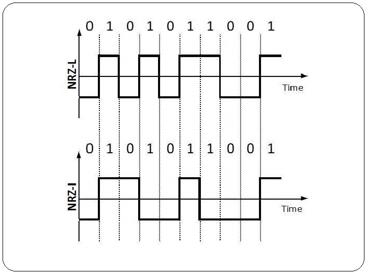
Line Coding Schemes: Polar encoding scheme uses multiple voltage levels to represent binary values. Polar encodings is available in four types: Polar Non-Return to Zero (Polar NRZ): It uses two different voltage levels to represent binary values. Generally, positive voltage represents 1 and negative value represents 0. It is also NRZ because there is no rest condition. NRZ scheme has two variants: NRZ-L and NRZ-I. NRZ-L changes voltage level at when a different bit is encountered whereas NRZ-I changes voltage when a 1 is encountered.

Return to Zero (RZ) Problem with NRZ is that the receiver cannot conclude when a bit ended and when the next bit is started, in case when sender and receiver’s clock are not synchronized. RZ uses three voltage levels, positive voltage to represent 1, negative voltage to represent 0 and zero voltage for none. Signals change during bits not between bits.

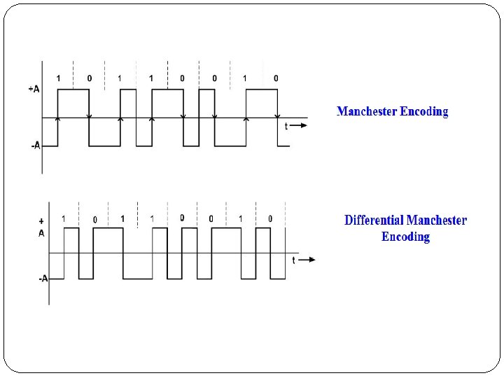
Manchester This encoding scheme is a combination of RZ and NRZ-L. Bit time is divided into two halves. It transits in the middle of the bit and changes phase when a different bit is encountered. Differential Manchester This encoding scheme is a combination of RZ and NRZ-I. It also transit at the middle of the bit but changes phase only when 1 is encountered.

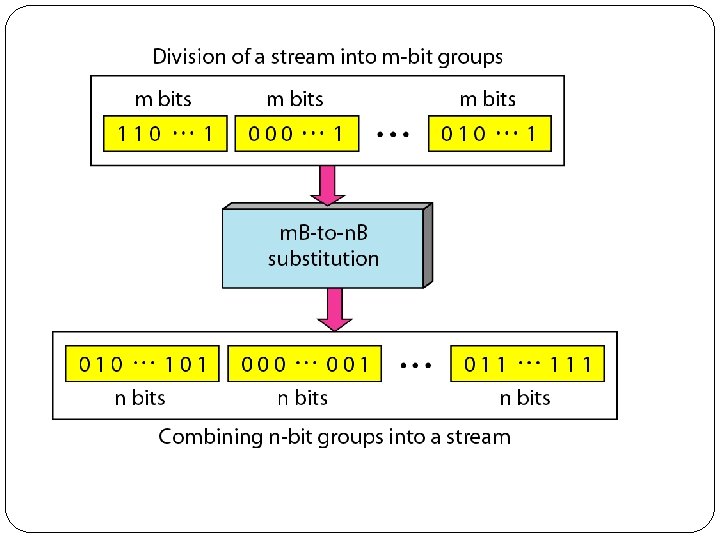
Block Coding To ensure accuracy (Synchronization/ error detection) of the received data frame redundant bits are used. For example, in even-parity, one parity bit is added to make the count of 1 s in the frame even. This way the original number of bits is increased. It is called Block Coding. Block coding is represented by slash notation, m. B/n. B. Means, m-bit block is substituted with n-bit block where n > m. Block coding involves three steps: Division: Original bit sequence is divided into groups of m bits. Substitution: The m-bit group is substituted for an n-bit group.

Scrambling This process substitutes long zero level pulses with a combination of different levels of pulses for providing synchronization. Two important techniques used in scrambling are: B 8 ZS HDB 3

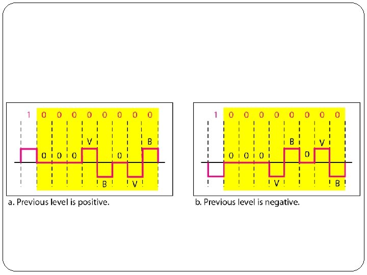
B 8 ZS: B: Bipolar, a non-zero voltage 8 ZS: 8 -Zero Substitution Eight consecutive zero level voltages are replaced by sequence 000 VB V: Violation, a non-zero voltage V indicates same polarity as the polarity of previous non-zero pulse B means polarity opposite to the polarity of previous non-zero pulse

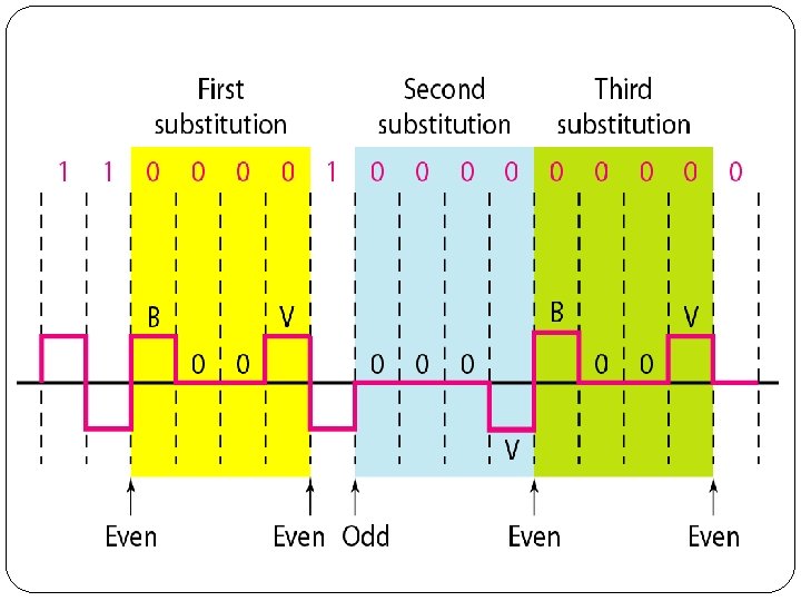
HDB 3: Stands for High-density bipolar 3 -zero (HDB 3) In this technique, which is more conservative than B 8 ZS, four consecutive zero-level voltages are replaced with a sequence of 000 V or B 00 V. The reason for two different substitutions is to maintain the even number of nonzero pulses after each substitution.

Digital-to-analog Conversion

When data from one computer is sent to another via some analog carrier, it is first converted into analog signals. Analog signals are modified to reflect digital data. An analog signal is characterized by its amplitude, frequency, and phase.

Aspects of Digital-to-Analog Conversion Information/ Data Element: Smallest piece of information Signal Element: Smallest unit of a signal that is constant Data Rate: Signal rate (baud rate) that is no. of bits per sec. Bandwidth: The bandwidth for analog transmission of digital data is proportional to the signal rate. FSK is exception. Carrier Signal: A high frequency signal which acts as a base for

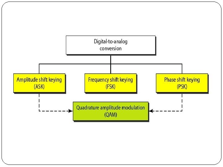
There are three kinds of digital-to-analog conversions: Amplitude Shift Keying (ASK) Frequency Shift Keying (FSK) Phase Shift Keying (PSK) Quadrature Amplitude Modulation(QAM)

1. Amplitude Shift Keying In this conversion technique, the amplitude of analog carrier signal is modified to reflect binary data. When binary data represents digit 1, the amplitude is held; otherwise it is set to 0. Both frequency and phase remain same as in the

2. Frequency Shift Keying In this conversion technique, the frequency of the analog carrier signal is modified to reflect binary data. This technique uses two frequencies, f 1 and f 2. One of them, for example f 1, is chosen to represent binary digit 1 and the other one is used

3. Phase Shift Keying In this conversion scheme, the phase of the original carrier signal is altered to reflect the binary data. When a new binary symbol is encountered, the phase of the signal is altered. Amplitude and frequency of the original carrier signal is kept

4. Quadrature Amplitude Modulation Quadrature amplitude modulation is a combination of ASK and PSK. QAM is a signal in which two carriers shifted in phase by 90 degrees are modulated and the resultant output consists of both amplitude and phase variations. In view of the fact that both amplitude and phase variations are present it may also be considered as a mixture of amplitude and phase modulation.

Analog-to-analog Conversion

Analog-to-analog Conversion