Published by Elsevier Academic Press San Diego in

Published by Elsevier Academic Press (San Diego) in 2015 Advanced Topics in Forensic DNA Typing: Interpretation John M. Butler, Ph. D. National Institute of Standards and Technology Slides from figures in the book provided for teaching purposes http: //www. cstl. nist. gov/strbase/training/Figures-Advanced-Topics-Forensic-DNA-Typing-Interpretation. pptx

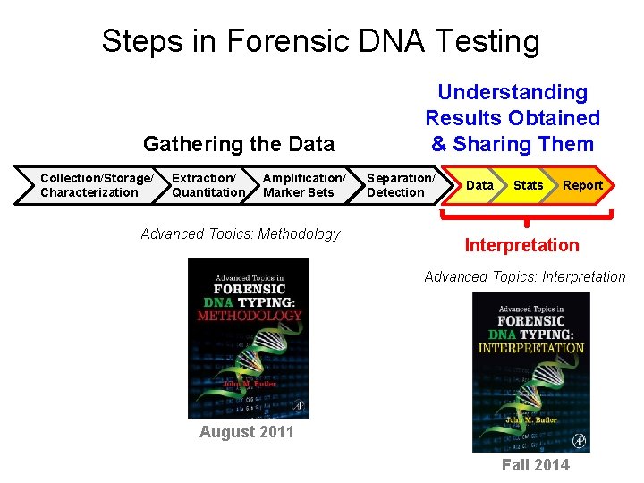
Steps in Forensic DNA Testing Gathering the Data Collection/Storage/ Characterization Extraction/ Quantitation Amplification/ Marker Sets Advanced Topics: Methodology Understanding Results Obtained & Sharing Them Separation/ Detection Data Stats Report Interpretation Advanced Topics: Interpretation August 2011 Fall 2014

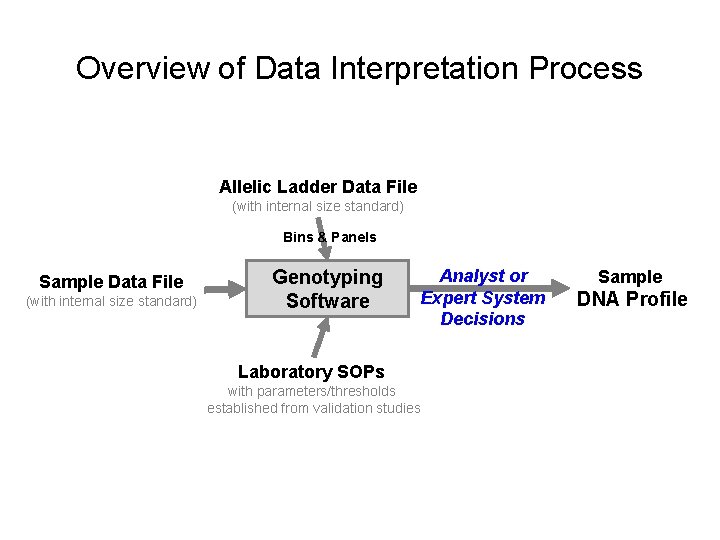
Overview of Data Interpretation Process Allelic Ladder Data File (with internal size standard) Bins & Panels Sample Data File (with internal size standard) Genotyping Software Analyst or Expert System Decisions Laboratory SOPs with parameters/thresholds established from validation studies Sample DNA Profile

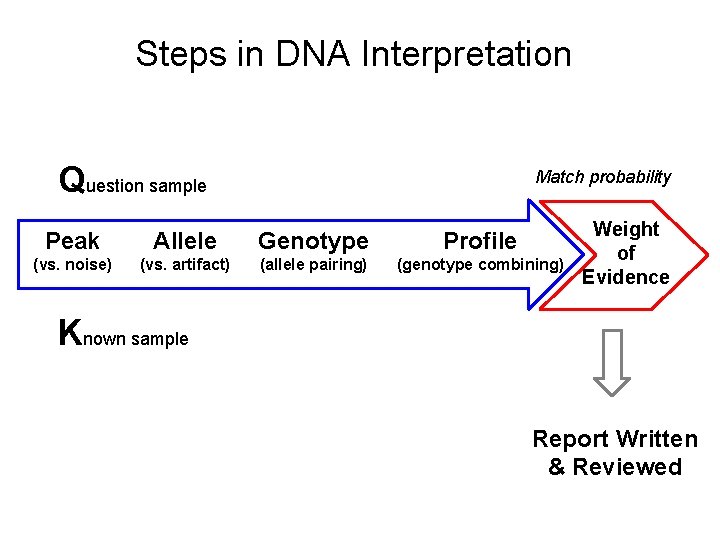
Steps in DNA Interpretation Question sample Match probability Peak Allele Genotype Profile (vs. noise) (vs. artifact) (allele pairing) (genotype combining) Weight of Evidence Known sample Report Written & Reviewed

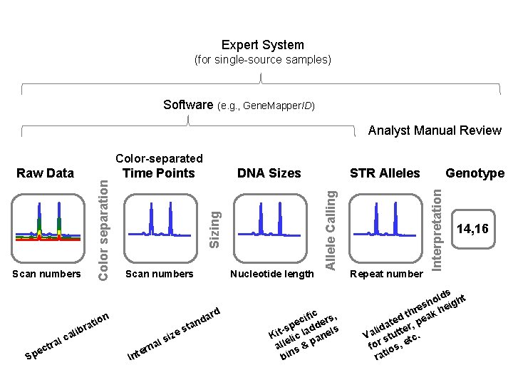
Expert System (for single-source samples) Software (e. g. , Gene. Mapper. ID) Analyst Manual Review Color-separated Sizing Scan numbers on ati e Sp r lib a c al ctr DNA Sizes Nucleotide length sta e siz I al n r nte rd a nd Genotype STR Alleles ific rs, c e e -sp ladd els t i K lic an e all s & p bin Repeat number Interpretation Time Points Allele Calling Scan numbers Color separation Raw Data 14, 16 lds ht o h es heig r h d t peak e t da tter, i l Va stu tc. for ios, e rat

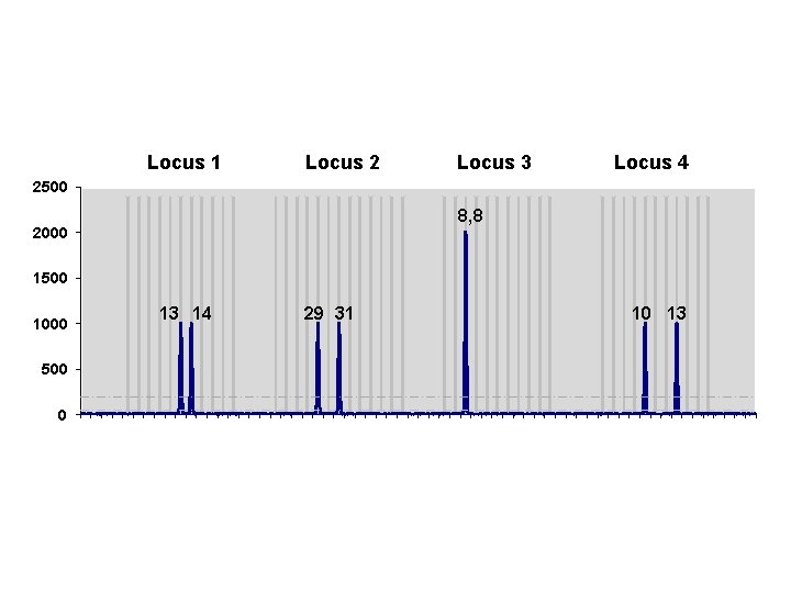
2500 Locus 2 Locus 3 Locus 4 1 14 27 40 53 Locus 1 8, 8 2000 1500 1000 13 14 29 31 10 13 500 0 1 2 3 4 5 6 7 8 9 10111213141516171819202122232425262728293031323334353637383940414243444546474849505152535455565758596061626364

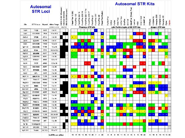
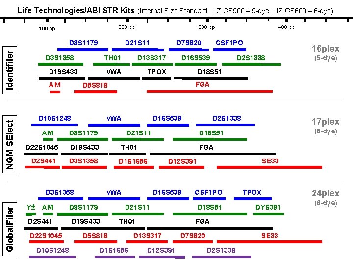
Life Technologies/ABI STR Kits (Internal Size Standard LIZ GS 500 – 5 -dye; LIZ GS 600 – 6 -dye) 200 bp 100 bp NGM SElect Identifiler D 8 S 1179 D 21 S 11 D 3 S 1358 D 19 S 433 AM D 13 S 317 v. WA TPOX D 8 S 1179 TH 01 D 2 S 441 D 3 S 1358 D 1 S 1656 D 2 S 441 D 22 S 1045 D 10 S 1248 D 16 S 539 D 2 S 1338 (5 -dye) D 2 S 1338 SE 33 D 12 S 391 D 21 S 11 TH 01 D 1 S 1656 (5 -dye) D 18 S 51 D 16 S 539 D 5 S 818 17 plex FGA v. WA D 19 S 433 16 plex D 18 S 51 D 21 S 11 D 8 S 1179 CSF 1 PO D 16 S 539 D 19 S 433 AM 400 bp FGA v. WA D 3 S 1358 Global. Filer TH 01 D 22 S 1045 Y± D 7 S 820 D 5 S 818 D 10 S 1248 AM 300 bp CSF 1 PO D 18 S 51 TPOX DYS 391 FGA D 13 S 317 D 12 S 391 D 7 S 820 SE 33 D 2 S 1338 24 plex (6 -dye)

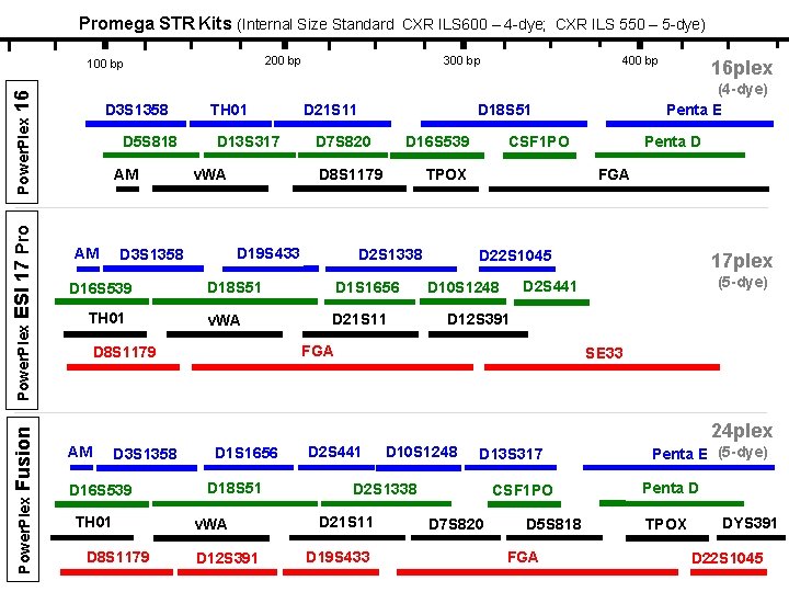
Promega STR Kits (Internal Size Standard CXR ILS 600 – 4 -dye; CXR ILS 550 – 5 -dye) 200 bp Power. Plex Fusion Power. Plex ESI 17 Pro Power. Plex 16 100 bp D 3 S 1358 D 5 S 818 AM AM TH 01 D 13 S 317 v. WA TH 01 D 21 S 11 400 bp D 16 S 539 D 8 S 1179 CSF 1 PO TPOX D 2 S 1338 D 18 S 51 D 1 S 1656 v. WA D 21 S 11 Penta D FGA D 22 S 1045 17 plex (5 -dye) D 2 S 441 D 10 S 1248 D 12 S 391 FGA D 8 S 1179 16 plex (4 -dye) Penta E D 18 S 51 D 7 S 820 D 19 S 433 D 3 S 1358 D 16 S 539 300 bp SE 33 24 plex AM D 3 S 1358 D 16 S 539 TH 01 D 8 S 1179 D 1 S 1656 D 18 S 51 v. WA D 12 S 391 D 2 S 441 D 10 S 1248 D 13 S 317 D 2 S 1338 D 21 S 11 D 19 S 433 CSF 1 PO D 7 S 820 D 5 S 818 FGA Penta E (5 -dye) Penta D TPOX DYS 391 D 22 S 1045

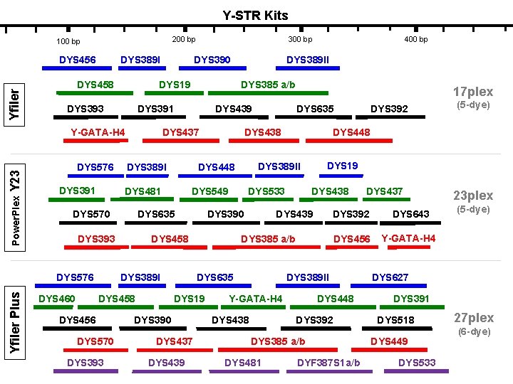
Y-STR Kits 200 bp 100 bp Yfiler DYS 456 DYS 389 I DYS 458 Power. Plex Y 23 DYS 391 DYS 389 I DYS 393 DYS 458 DYS 456 DYS 570 DYS 393 DYS 390 DYS 437 DYS 439 DYS 438 DYS 643 DYS 456 Y-GATA-H 4 DYS 389 II DYS 448 Y-GATA-H 4 DYS 438 DYS 392 DYS 385 a/b DYS 481 DYS 437 DYS 392 DYS 385 a/b DYS 19 (5 -dye) DYS 19 DYS 439 DYS 635 DYS 392 DYS 448 DYS 533 DYS 458 DYS 389 I DYS 635 DYS 389 II DYS 549 DYS 635 17 plex DYS 438 DYS 448 DYS 481 DYS 576 Yfiler Plus DYS 439 DYS 437 DYS 570 DYS 460 DYS 385 a/b DYS 391 Y-GATA-H 4 400 bp DYS 389 II DYS 390 DYS 19 DYS 393 DYS 576 300 bp DYF 387 S 1 a/b 23 plex (5 -dye) DYS 627 DYS 391 DYS 518 DYS 449 DYS 533 27 plex (6 -dye)

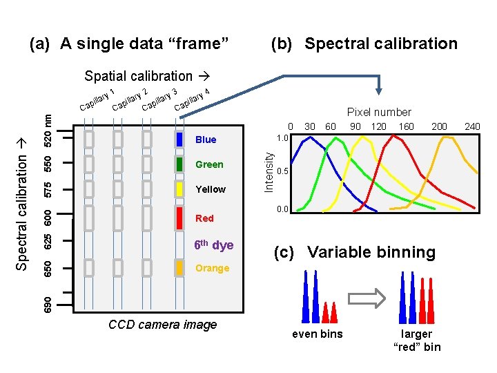
(a) A single data “frame” (b) Spectral calibration Spatial calibration 1 ry Pixel number 0 6 th dye Orange Yellow Red Intensity Green 30 60 90 120 160 200 1. 0 Blue 625 600 575 550 520 nm Ca 650 Ca 2 3 4 ry ary l l i i p p Ca Ca a pill 0. 5 0. 0 (c) Variable binning 690 Spectral calibration a pill CCD camera image even bins larger “red” bin 240

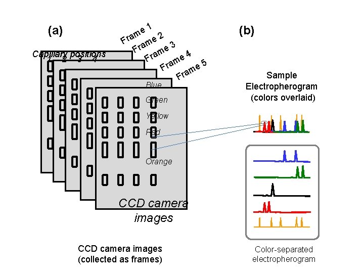
(a) Capillary positions 1 2 3 4 e 1 m 2 Fra me 3 Fra me 4 e Fra m 5 e Fra m Fra Blue Green (b) Sample Electropherogram (colors overlaid) Yellow Red Orange CCD camera images (collected as frames) Color-separated electropherogram

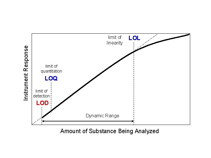
Instrument Response limit of linearity LOL limit of quantitation LOQ limit of detection LOD Dynamic Range Amount of Substance Being Analyzed

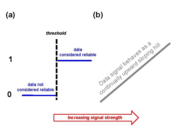
(a) (b) threshold data considered reliable 1 0 data not considered reliable l a il s h a g s in e v op a h sl e b rd l a wa n g up i s lly a t a a D inu t n co Increasing signal strength

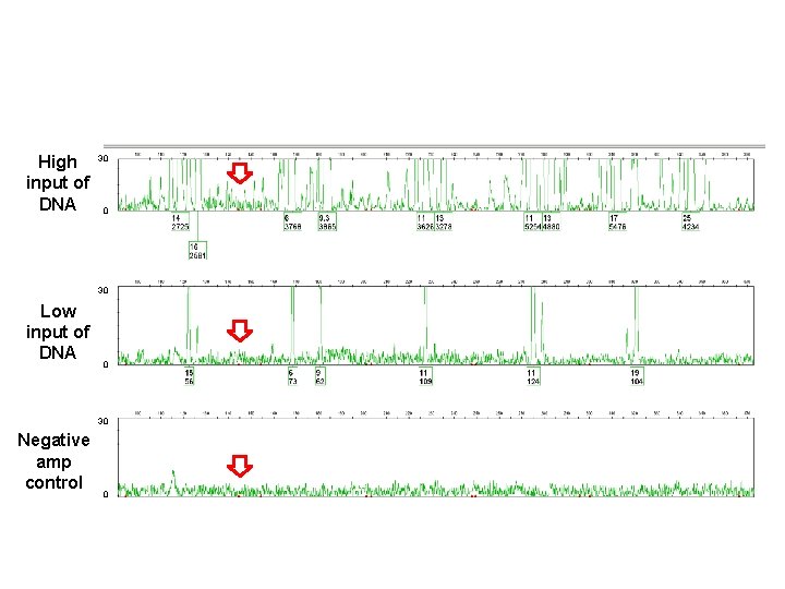
High 30 input of DNA 0 30 Low input of DNA 0 30 Negative amp control 0

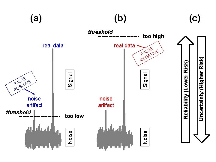
(b) threshold noise artifact too low Uncertainty (Higher Risk) Signal SE E L FA ATIV G NE Noise noise artifact threshold Noise SE E L FA ITIV S PO too high real data (c) Reliability (Lower Risk) (a)

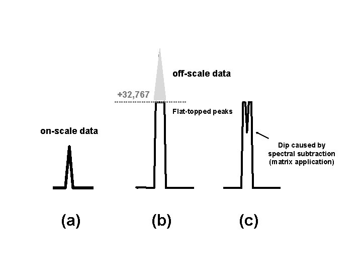
off-scale data +32, 767 Flat-topped peaks on-scale data Dip caused by spectral subtraction (matrix application) (a) (b) (c)

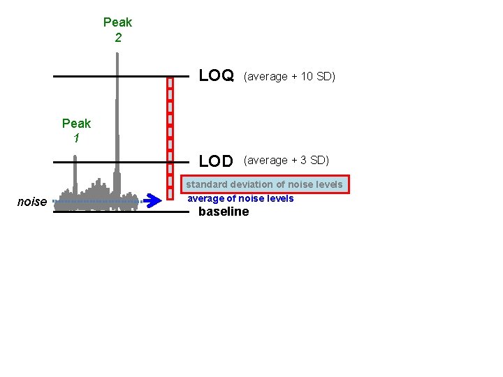
Peak 2 LOQ (average + 10 SD) LOD (average + 3 SD) Peak 1 noise standard deviation of noise levels average of noise levels baseline

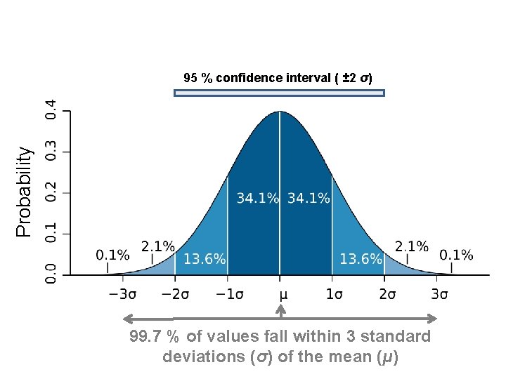
Probability 95 % confidence interval ( ± 2 σ) 99. 7 % of values fall within 3 standard deviations (σ) of the mean (μ)

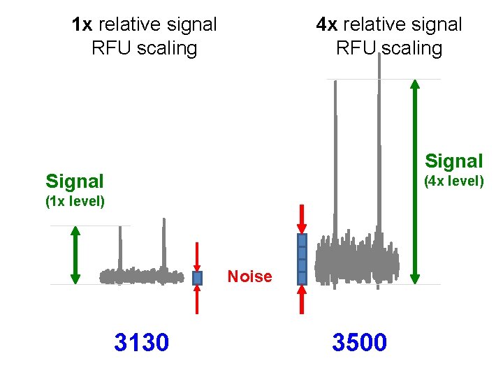
1 x relative signal RFU scaling 4 x relative signal RFU scaling Signal (4 x level) (1 x level) Noise 3130 3500

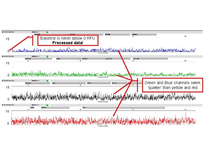
15 Baseline is never below 0 RFU Processed data! 0 15 0 Green and Blue channels seem ‘quieter’ than yellow and red

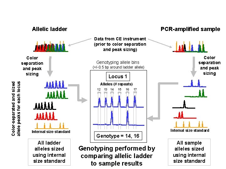
Allelic ladder PCR-amplified sample Data from CE instrument (prior to color separation and peak sizing) Color-separated and sized allele peaks for each locus Color separation and peak sizing Genotyping allele bins (+/-0. 5 bp around ladder allele) Locus 1 Color separation and peak sizing Alleles (# repeats) 12 Internal size standard All ladder alleles sized using internal size standard 13 14 15 16 17 Internal size standard Genotype = 14, 16 Genotyping performed by comparing allelic ladder to sample results All sample alleles sized using internal size standard

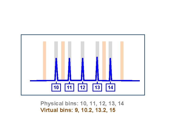
10 11 12 13 14 Physical bins: 10, 11, 12, 13, 14 Virtual bins: 9, 10. 2, 13. 2, 15

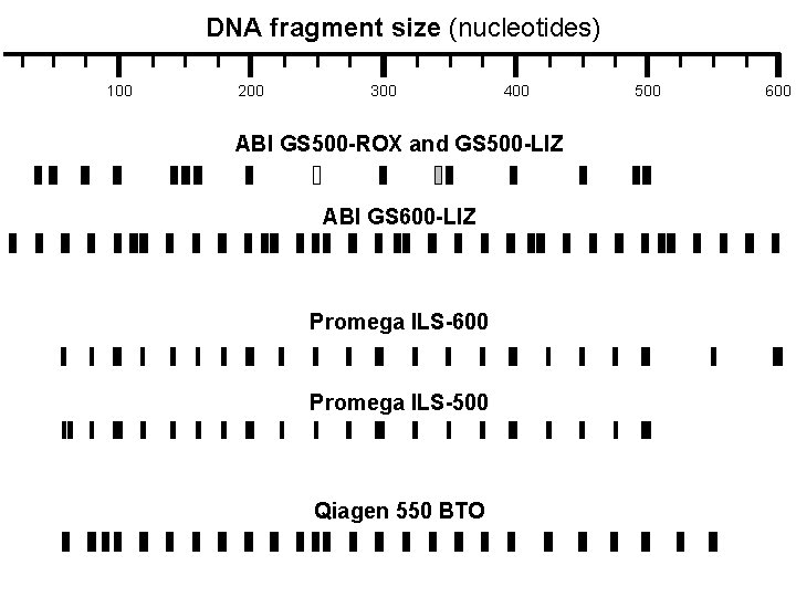
DNA fragment size (nucleotides) 100 200 300 400 ABI GS 500 -ROX and GS 500 -LIZ ABI GS 600 -LIZ Promega ILS-600 Promega ILS-500 Qiagen 550 BTO 500 600

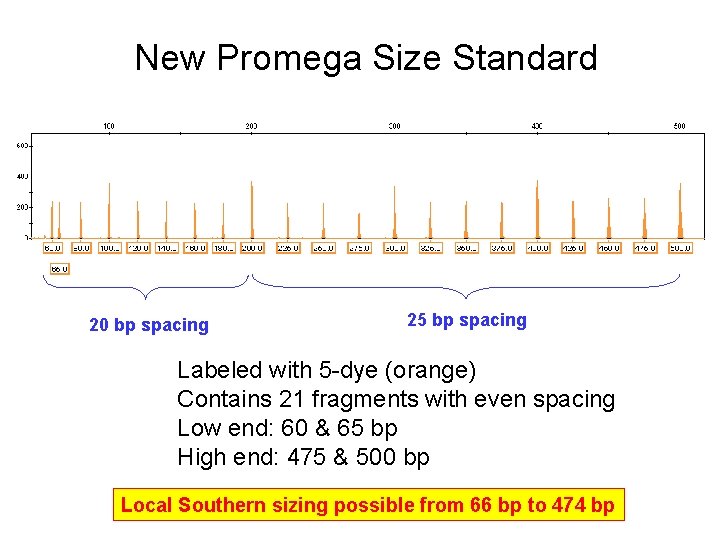
New Promega Size Standard 20 bp spacing 25 bp spacing Labeled with 5 -dye (orange) Contains 21 fragments with even spacing Low end: 60 & 65 bp High end: 475 & 500 bp Local Southern sizing possible from 66 bp to 474 bp

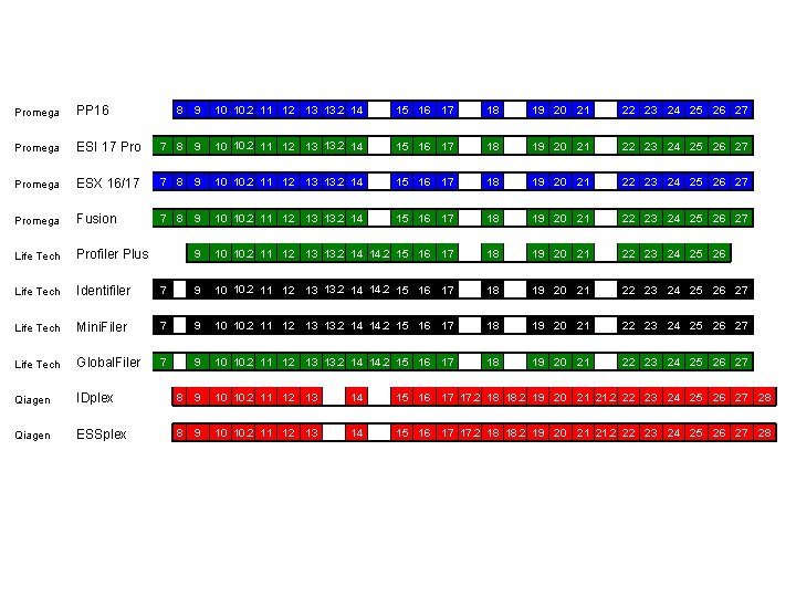
Promega PP 16 Promega 8 9 10 10. 2 11 12 13 13. 2 14 15 16 17 18 19 20 21 22 23 24 25 26 27 ESI 17 Pro 7 8 9 10 10. 2 11 12 13 13. 2 14 15 16 17 18 19 20 21 22 23 24 25 26 27 Promega ESX 16/17 7 8 9 10 10. 2 11 12 13 13. 2 14 15 16 17 18 19 20 21 22 23 24 25 26 27 Promega Fusion 7 8 9 10 10. 2 11 12 13 13. 2 14 15 16 17 18 19 20 21 22 23 24 25 26 27 Life Tech Profiler Plus 9 10 10. 2 11 12 13 13. 2 14 14. 2 15 16 17 18 19 20 21 22 23 24 25 26 Life Tech Identifiler 7 9 10 10. 2 11 12 13 13. 2 14 14. 2 15 16 17 18 19 20 21 22 23 24 25 26 27 Life Tech Mini. Filer 7 9 10 10. 2 11 12 13 13. 2 14 14. 2 15 16 17 18 19 20 21 22 23 24 25 26 27 Life Tech Global. Filer 7 9 10 10. 2 11 12 13 13. 2 14 14. 2 15 16 17 18 19 20 21 22 23 24 25 26 27 Qiagen IDplex 8 9 10 10. 2 11 12 13 14 15 16 17 17. 2 18 18. 2 19 20 21 21. 2 22 23 24 25 26 27 28 Qiagen ESSplex 8 9 10 10. 2 11 12 13 14 15 16 17 17. 2 18 18. 2 19 20 21 21. 2 22 23 24 25 26 27 28

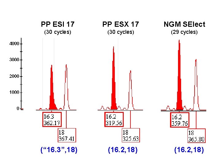
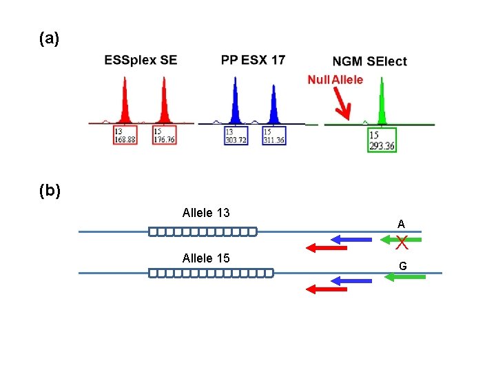
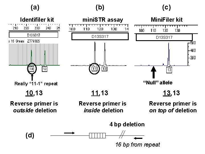
PP ESI 17 PP ESX 17 NGM SElect (30 cycles) (29 cycles) (“ 16. 3”, 18) (16. 2, 18)

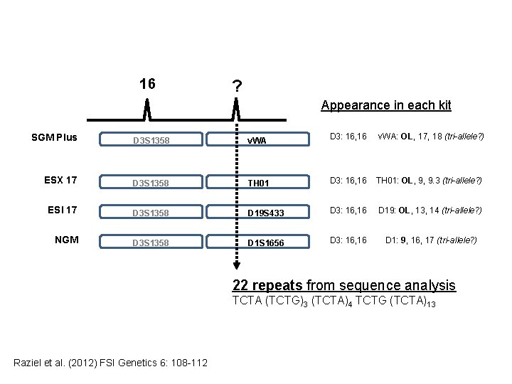
16 ? Appearance in each kit SGM Plus D 3 S 1358 v. WA D 3: 16, 16 v. WA: OL, 17, 18 (tri-allele? ) ESX 17 D 3 S 1358 TH 01 D 3: 16, 16 TH 01: OL, 9, 9. 3 (tri-allele? ) ESI 17 D 3 S 1358 D 19 S 433 D 3: 16, 16 D 19: OL, 13, 14 (tri-allele? ) NGM D 3 S 1358 D 1 S 1656 D 3: 16, 16 D 1: 9, 16, 17 (tri-allele? ) 22 repeats from sequence analysis TCTA (TCTG)3 (TCTA)4 TCTG (TCTA)13 Raziel et al. (2012) FSI Genetics 6: 108 -112

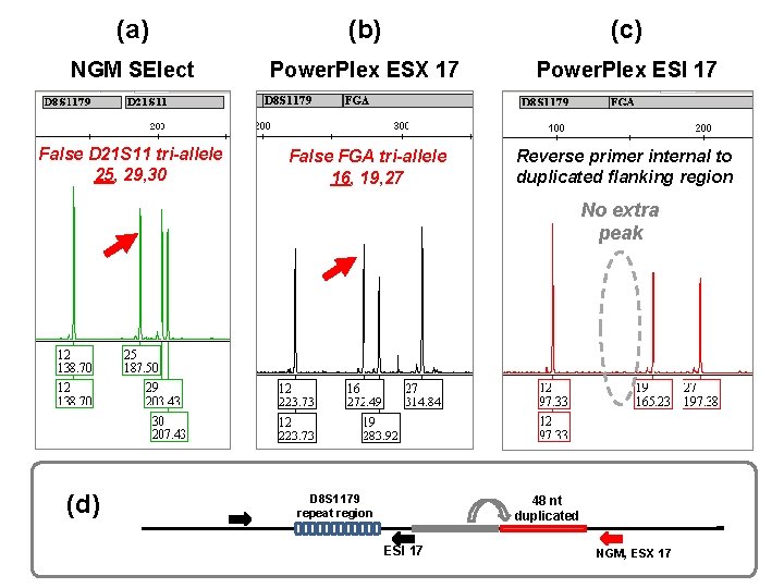
(a) (b) (c) NGM SElect Power. Plex ESX 17 Power. Plex ESI 17 False D 21 S 11 tri-allele 25, 29, 30 False FGA tri-allele 16, 19, 27 Reverse primer internal to duplicated flanking region No extra peak (d) D 8 S 1179 repeat region 48 nt duplicated ESI 17 NGM, ESX 17

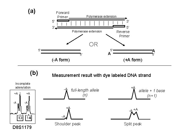
(a) Forward Primer Polymerase extension 5’ 3’ 3’ 5’ Reverse Primer Polymerase extension OR 5’ 5’ (-A form) (b) Incomplete adenylation +A -A +A A A 5’ 5’ (+A form) Measurement result with dye labeled DNA strand -A full-length allele +A (n) allele + 1 base (n+1) -A +A Shoulder peak Split peak -A D 8 S 1179

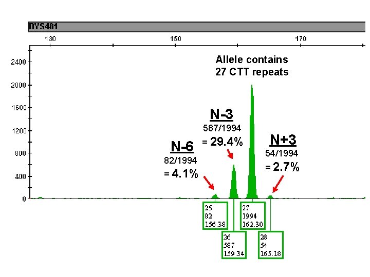
Allele contains 27 CTT repeats N-3 587/1994 N-6 82/1994 = 4. 1% = 29. 4% N+3 54/1994 = 2. 7%

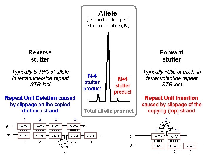
Allele (tetranucleotide repeat, size in nucleotides, N) Reverse stutter Forward stutter Typically 5 -15% of allele in tetranucleotide repeat STR loci N-4 stutter product Repeat Unit Deletion caused by slippage on the copied (bottom) strand N+4 stutter product Total allelic product 1 2 3 5’ GATA 3’ CTAT CTAT 1 2 3 5 6 Typically <2% of allele in tetranucleotide repeat STR loci Repeat Unit Insertion caused by slippage of the copying (top) strand 5 C T A 4 T 2’ 1 2 5’ GATA 3’ CTAT 1 2 3

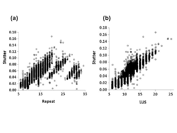
t pe a re e id le ot uc Tr i-n Hexa-nucleotide repeat

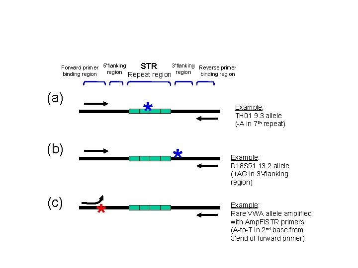
3’flanking Reverse primer STR Forward primer 5’flanking region binding region Repeat region binding region (a) * (b) (c) Example: TH 01 9. 3 allele (-A in 7 th repeat) * * Example: D 18 S 51 13. 2 allele (+AG in 3’-flanking region) Example: Rare VWA allele amplified with Amp. Fl. STR primers (A-to-T in 2 nd base from 3’end of forward primer)

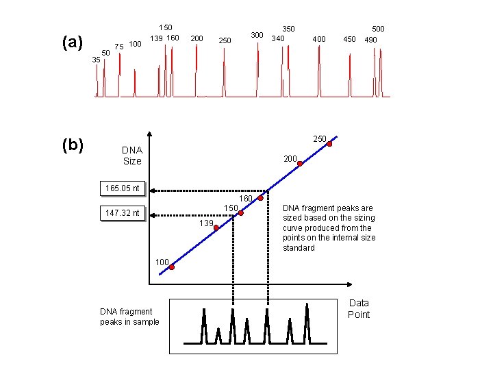
(a) 35 (b) 50 75 100 150 139 160 200 250 300 350 340 400 450 500 490 250 DNA Size 200 165. 05 nt 160 150 147. 32 nt 139 DNA fragment peaks are sized based on the sizing curve produced from the points on the internal size standard 100 DNA fragment peaks in sample Data Point

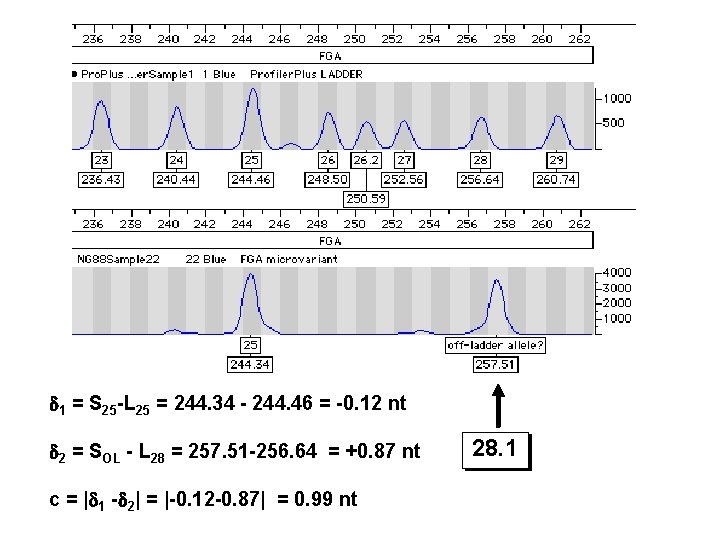
1 = S 25 -L 25 = 244. 34 - 244. 46 = -0. 12 nt 2 = SOL - L 28 = 257. 51 -256. 64 = +0. 87 nt c = | 1 - 2| = |-0. 12 -0. 87| = 0. 99 nt 28. 1

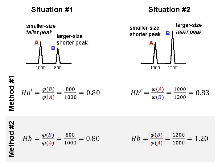
Situation #1 smaller-size taller peak A Method #2 Method #1 1000 B larger-size shorter peak Situation #2 smaller-size shorter peak B larger-size taller peak A 800 1000 1200

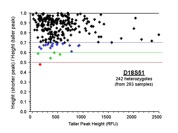
Height (shorter peak) / Height (taller peak) 1. 0 0. 9 0. 8 0. 7 0. 6 0. 5 0. 4 D 18 S 51 0. 3 242 heterozygotes (from 283 samples) 0. 2 0. 1 0. 0 0 500 1000 1500 Taller Peak Height (RFU) 2000 2500

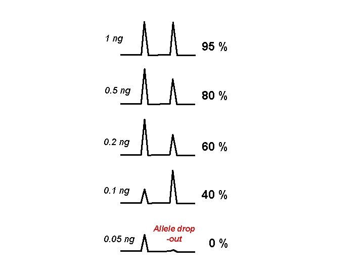
1 ng 95 % 0. 5 ng 80 % 0. 2 ng 60 % 0. 1 ng 40 % 0. 05 ng Allele drop -out 0 %

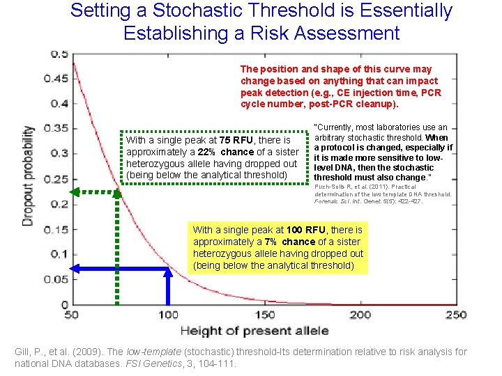
Setting a Stochastic Threshold is Essentially Drop Out Probability as a Function of Surviving Sister Allele Peak Height Establishing a Risk Assessment The position and shape of this curve may change based on anything that can impact peak detection (e. g. , CE injection time, PCR cycle number, post-PCR cleanup). With a single peak at 75 RFU, there is approximately a 22% chance of a sister heterozygous allele having dropped out (being below the analytical threshold) “Currently, most laboratories use an arbitrary stochastic threshold. When a protocol is changed, especially if it is made more sensitive to lowlevel DNA, then the stochastic threshold must also change. ” Puch-Solis R, et al. (2011). Practical determination of the low template DNA threshold. Forensic Sci. Int. Genet. 5(5): 422 -427. With a single peak at 100 RFU, there is approximately a 7% chance of a sister heterozygous allele having dropped out (being below the analytical threshold) Gill, P. , et al. (2009). The low-template (stochastic) threshold-Its determination relative to risk analysis for national DNA databases. FSI Genetics, 3, 104 -111.

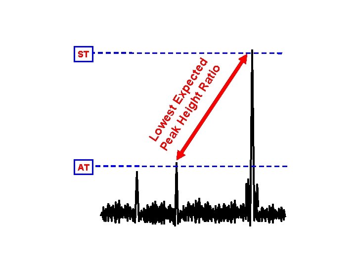
AT Lo Pe wes ak t E H eig xpe ht cte R d ati o ST

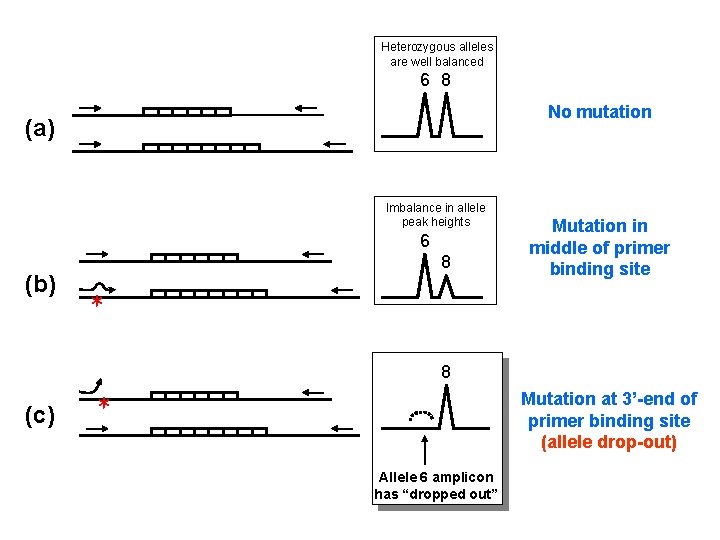
Heterozygous alleles are well balanced 6 8 No mutation (a) Imbalance in allele peak heights 6 (b) 8 Mutation in middle of primer binding site * 8 (c) * Mutation at 3’-end of primer binding site (allele drop-out) Allele 6 amplicon has “dropped out”

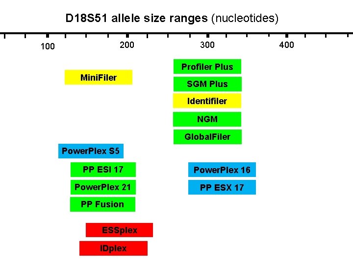
D 18 S 51 allele size ranges (nucleotides) 200 100 300 Profiler Plus Mini. Filer SGM Plus Identifiler NGM Global. Filer Power. Plex S 5 PP ESI 17 Power. Plex 16 Power. Plex 21 PP ESX 17 PP Fusion ESSplex IDplex 400

(a) (b) Allele 13 Allele 15 A X G

(a) Identifiler kit (b) (c) Mini. Filer kit mini. STR assay D 13 S 317 “Null” allele Really “ 11 -1” repeat 10, 13 Reverse primer is outside deletion 11, 13 13, 13 Reverse primer is inside deletion Reverse primer is on top of deletion 4 bp deletion (d) 16 bp from repeat

6 -FAM label (blue channel) VIC label (green channel) NED label (yellow channel) PET label (red channel)

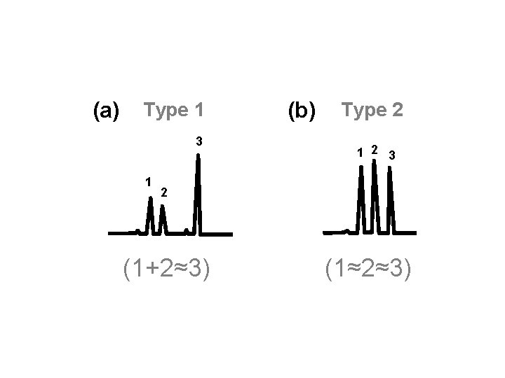
(a) Type 1 3 1 (b) Type 2 1 2 3 2 (1+2≈3) (1≈2≈3)

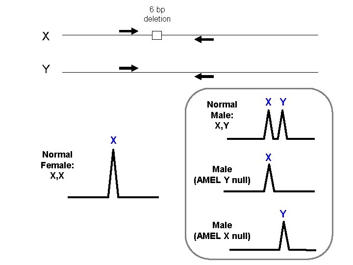
6 bp deletion X Y Normal Male: X, Y X Normal Female: X, X X Male (AMEL Y null) Y Male (AMEL X null)

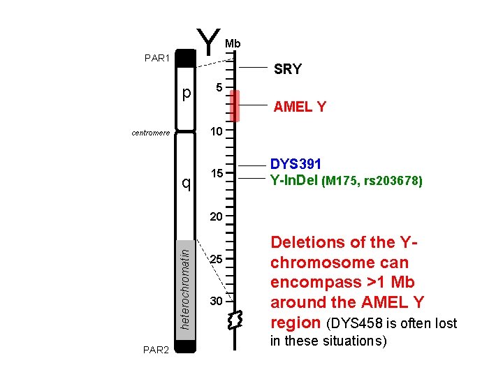
Y PAR 1 p Mb SRY 5 AMEL Y 10 centromere q 15 DYS 391 Y-In. Del (M 175, rs 203678) heterochromatin 20 PAR 2 25 30 Deletions of the Ychromosome can encompass >1 Mb around the AMEL Y region (DYS 458 is often lost in these situations)

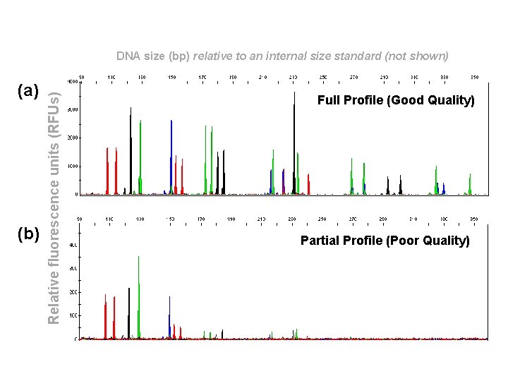
(a) (b) Relative fluorescence units (RFUs) DNA size (bp) relative to an internal size standard (not shown) Full Profile (Good Quality) Partial Profile (Poor Quality)

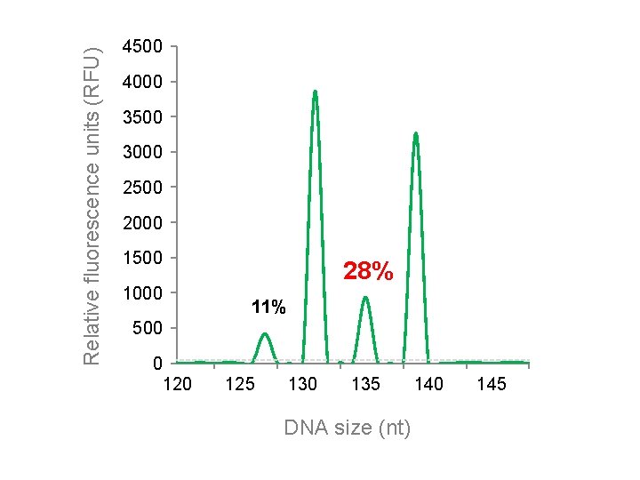
Relative fluorescence units (RFU) 4500 4000 3500 3000 2500 2000 1500 1000 28% 11% 500 0 125 130 135 DNA size (nt) 140 145

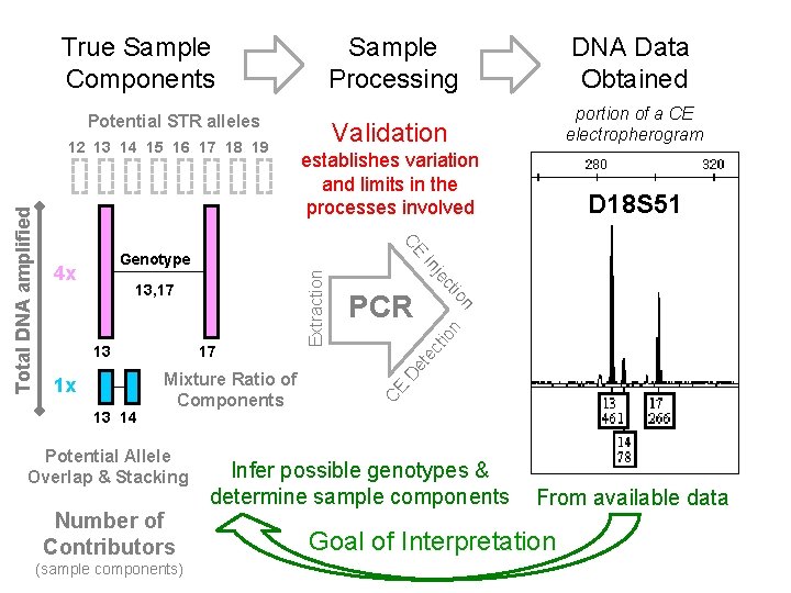
True Sample Components Sample Processing DNA Data Obtained Validation portion of a CE electropherogram establishes variation and limits in the processes involved D 18 S 51 Potential STR alleles Potential Allele Overlap & Stacking Number of Contributors (sample components) CE D et ec tio n n 13 14 Mixture Ratio of Components PCR io 1 x 17 ct 13 je 13, 17 Extraction Genotype 4 x In CE Total DNA amplified 12 13 14 15 16 17 18 19 Infer possible genotypes & determine sample components From available data Goal of Interpretation

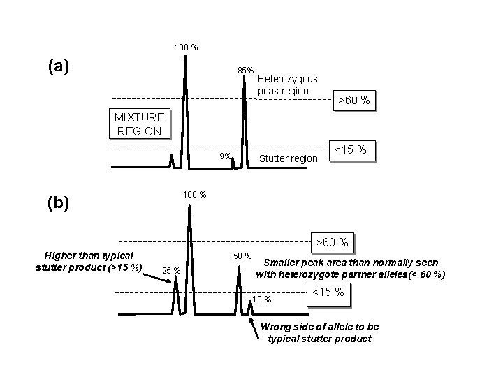
100 % (a) 85% Heterozygous peak region >60 % MIXTURE REGION 9% Stutter region <15 % 100 % (b) >60 % Higher than typical stutter product (>15 %) 50 % 25 % Smaller peak area than normally seen with heterozygote partner alleles(< 60 %) 10 % <15 % Wrong side of allele to be typical stutter product

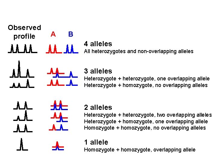
Observed profile A B 4 alleles All heterozygotes and non-overlapping alleles 3 alleles Heterozygote + heterozygote, one overlapping allele Heterozygote + homozygote, no overlapping alleles 2 alleles Heterozygote + heterozygote, two overlapping alleles Heterozygote + homozygote, one overlapping allele Homozygote + homozygote, no overlapping alleles 1 allele Homozygote + homozygote, overlapping allele

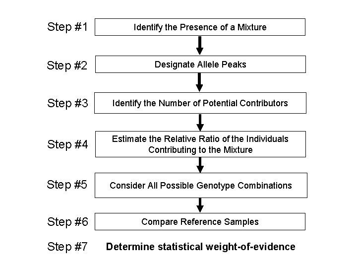
Step #1 Identify the Presence of a Mixture Step #2 Designate Allele Peaks Step #3 Identify the Number of Potential Contributors Step #4 Estimate the Relative Ratio of the Individuals Contributing to the Mixture Step #5 Consider All Possible Genotype Combinations Step #6 Compare Reference Samples Step #7 Determine statistical weight-of-evidence

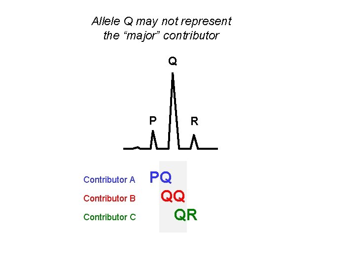
Allele Q may not represent the “major” contributor Q P Contributor A Contributor B Contributor C R PQ QQ QR

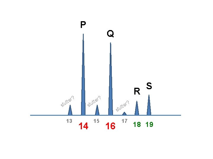
P tte u t s r? 13 Q R r? tte u t s 14 15 S ? er t t u st 16 17 18 19

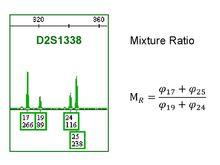
D 2 S 1338 Mixture Ratio

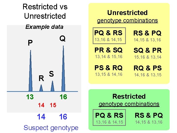
Restricted vs Unrestricted Example data Q P R S 13 16 14 15 14 16 Suspect genotype Unrestricted genotype combinations PQ & RS RS & PQ 13, 16 & 14, 15 & 13, 16 PR & SQ SQ & PR 13, 14 & 15, 16 & 13, 14 PS & RQ RQ & PS 13, 15 & 14, 16 & 13, 15 Restricted genotype combinations PQ & RS RS & PQ 13, 16 & 14, 15 & 13, 16

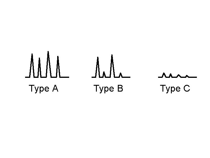
Type A Type B Type C

Is the sample a mixture? >2 alleles at a locus, except trialleles? NO Single Source DNA Sample Likelihood Ratio [LR] Determine STR profile and compute RMP YES Probability of Exclusion [CPE] “RMNE” Mixed DNA Sample Differentiate a Major/Minor Component? NO YES TYPE B Determine component profile(s) and compute RMP for major Stochastic Effects ? Possible Low Level DNA) ? YES TYPE C A biostatistical analysis should not be performed NO NO Assume number of contributors? TYPE A A biostatistical analysis must be performed

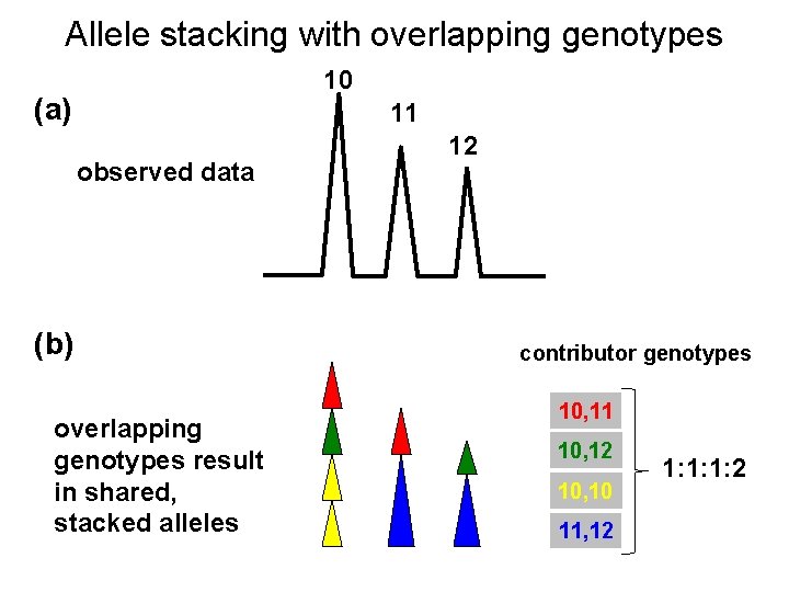
Allele stacking with overlapping genotypes 10 (a) 11 observed data (b) overlapping genotypes result in shared, stacked alleles 12 contributor genotypes 10, 11 10, 12 10, 10 11, 12 1: 1: 1: 2

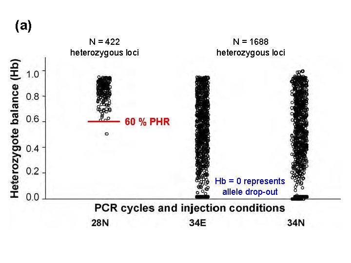
(a) N = 422 heterozygous loci N = 1688 heterozygous loci 60 % PHR Hb = 0 represents allele drop-out

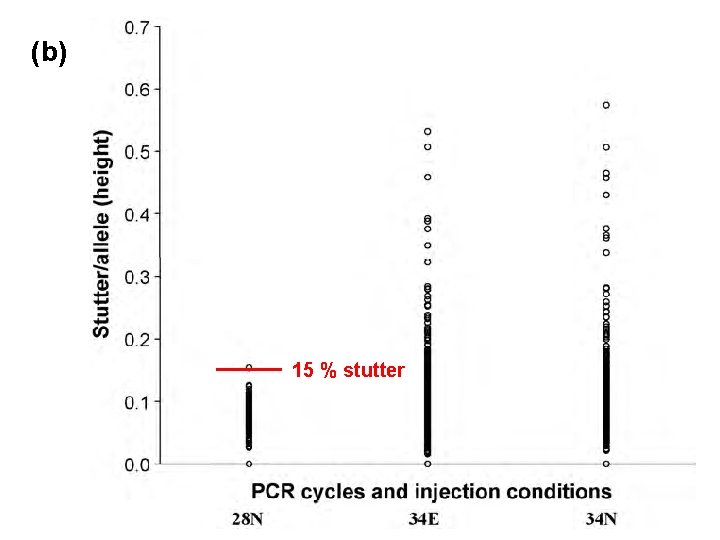
(b) 15 % stutter

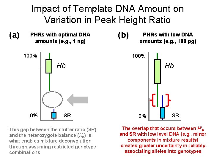
Impact of Template DNA Amount on Variation in Peak Height Ratio (a) PHRs with optimal DNA amounts (e. g. , 1 ng) 100% (b) PHRs with low DNA amounts (e. g. , 100 pg) 100% Hb 0% SR This gap between the stutter ratio (SR) and the heterozygote balance (Hb) is what enables mixture deconvolution through assuming restricted genotype combinations Hb 0% SR The overlap that occurs between H′b and SR with low level DNA (e. g. , minor components in mixture results) creates greater uncertainty in reliably associating alleles into genotypes

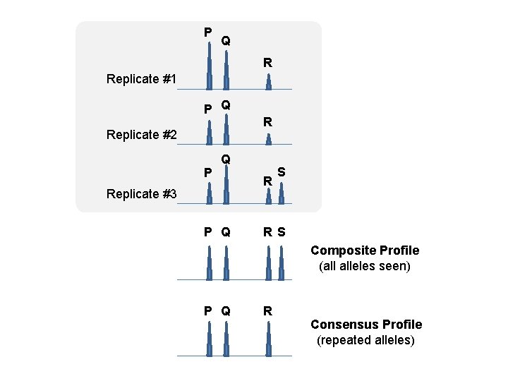
P Q R Replicate #1 P Q Replicate #2 P R Q Replicate #3 P Q R S Composite Profile (all alleles seen) P Q R Consensus Profile (repeated alleles)

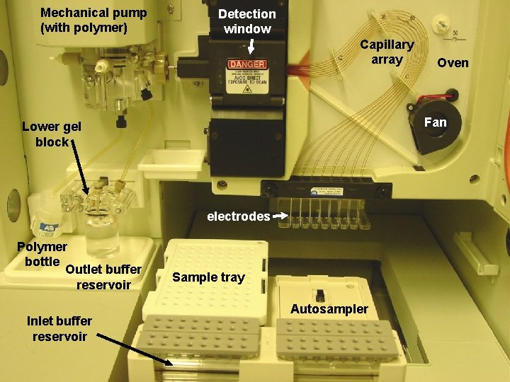
Mechanical pump (with polymer) Detection window Capillary array Fan Lower gel block electrodes Polymer bottle Outlet buffer reservoir Inlet buffer reservoir Oven Sample tray Autosampler

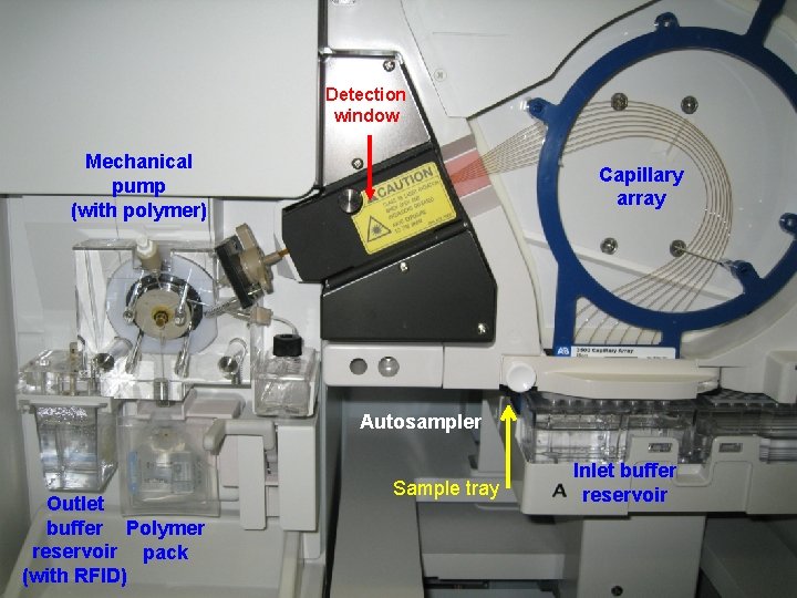
Detection window Mechanical pump (with polymer) Capillary array Autosampler Outlet buffer Polymer reservoir pack (with RFID) Sample tray Inlet buffer reservoir

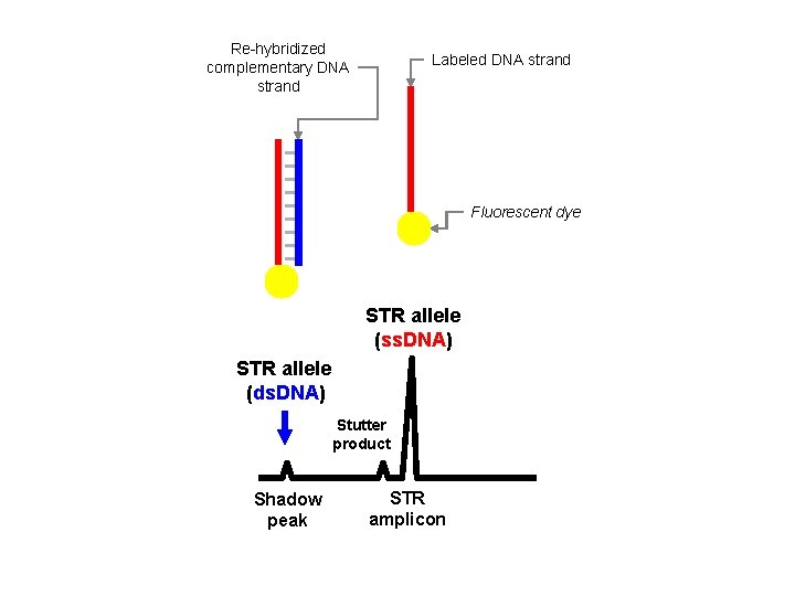
Re-hybridized complementary DNA strand Labeled DNA strand Fluorescent dye STR allele (ss. DNA) STR allele (ds. DNA) Stutter product Shadow peak STR amplicon

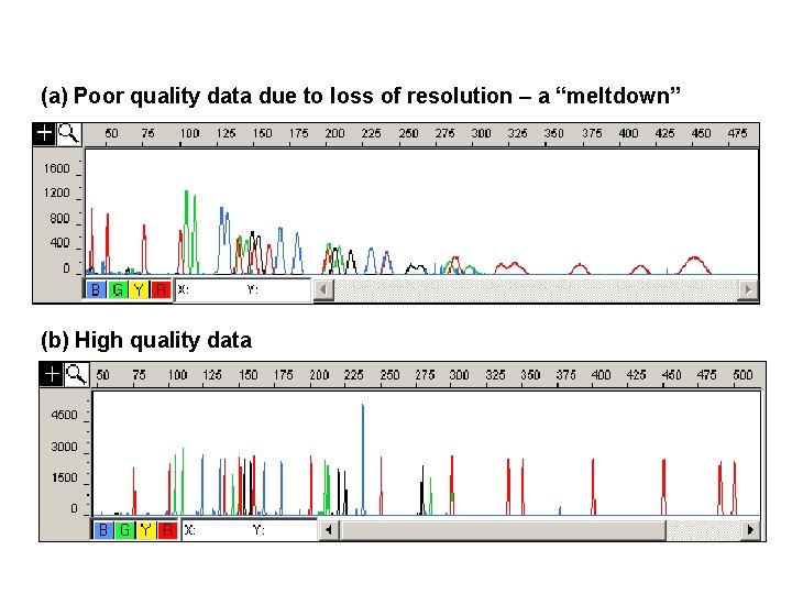
(a) Poor quality data due to loss of resolution – a “meltdown” (b) High quality data

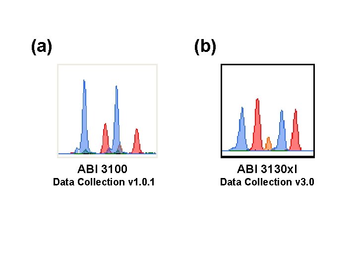
(a) (b) ABI 3100 ABI 3130 xl Data Collection v 1. 0. 1 Data Collection v 3. 0

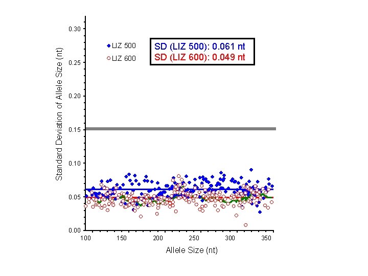
Standard Deviation of Allele Size (nt) 0. 30 LIZ 500 0. 25 LIZ 600 SD (LIZ 500): 0. 061 nt SD (LIZ 600): 0. 049 nt s(LIZ 500): 0. 061 bp 0. 20 s(LIZ 600): 0. 049 bp 0. 15 0. 10 0. 05 0. 00 150 200 250 Allele Size (nt) 300 350

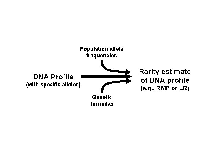
Population allele frequencies Rarity estimate of DNA profile DNA Profile (with specific alleles) (e. g. , RMP or LR) Genetic formulas

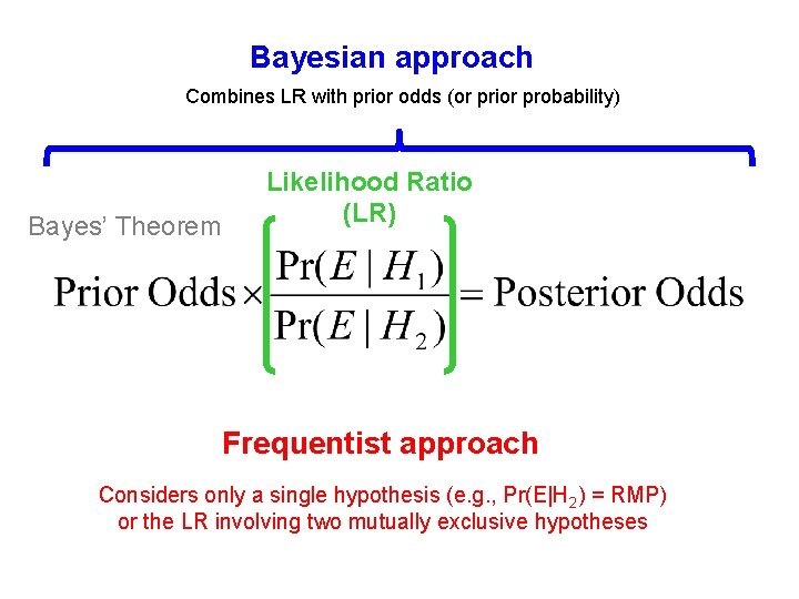
Bayesian approach Combines LR with prior odds (or prior probability) Bayes’ Theorem Likelihood Ratio (LR) Frequentist approach Considers only a single hypothesis (e. g. , Pr(E|H 2) = RMP) or the LR involving two mutually exclusive hypotheses

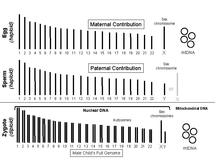
Egg (haploid) Sex chromosome Maternal Contribution Sperm (haploid) 1 2 3 4 5 6 7 8 9 10 11 12 13 14 15 16 17 18 19 20 21 22 Sex chromosome Paternal Contribution or 1 2 3 4 5 6 7 8 9 10 11 12 13 14 15 16 17 18 19 20 21 22 Nuclear DNA Zygote (diploid) mt. DNA X Autosomes Sex chromosomes 1 2 3 4 5 6 7 8 9 10 11 12 13 14 15 16 17 18 19 20 21 22 Male Child’s Full Genome Y XY X Mitochondrial DNA mt. DNA

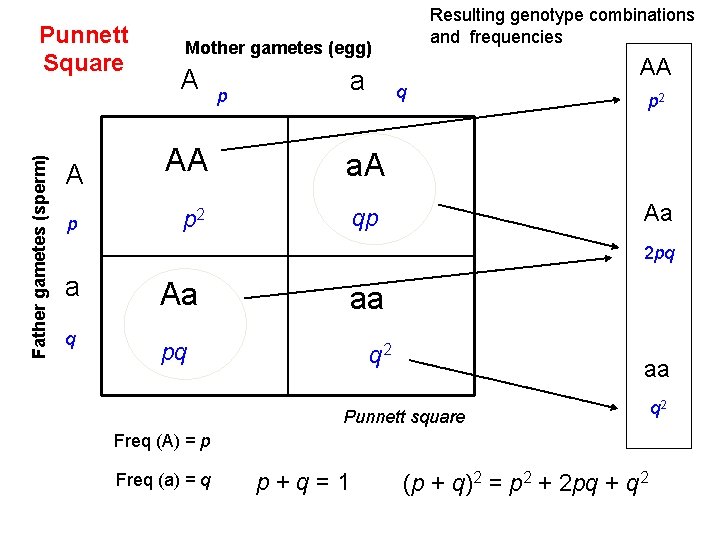
Father gametes (sperm) Punnett Square A p Resulting genotype combinations and frequencies Mother gametes (egg) A p a AA q AA a. A p 2 qp p 2 Aa 2 pq a q Aa aa pq q 2 aa Punnett square Freq (A) = p Freq (a) = q p + q = 1 (p + q)2 = p 2 + 2 pq + q 2

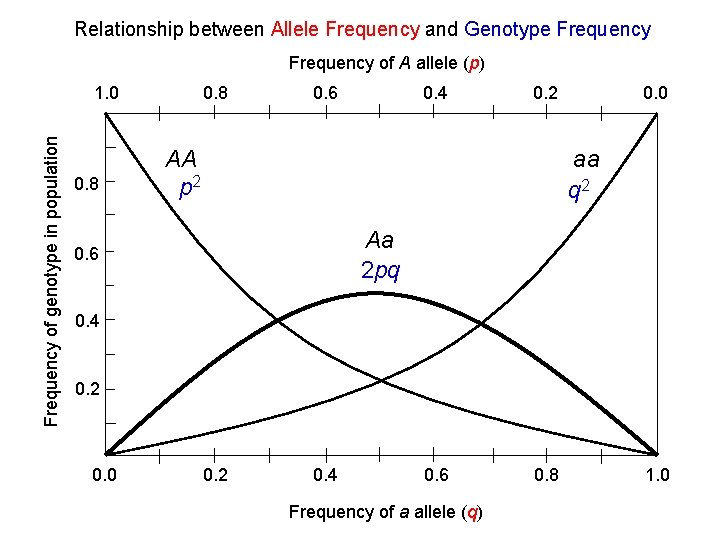
Relationship between Allele Frequency and Genotype Frequency of A allele (p) Frequency of genotype in population 1. 0 0. 8 0. 6 0. 4 0. 2 AA p 2 0. 0 aa q 2 Aa 2 pq 0. 6 0. 4 0. 2 0. 0 0. 2 0. 4 0. 6 Frequency of a allele (q) 0. 8 1. 0

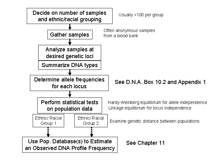
Decide on number of samples and ethnic/racial grouping Gather samples Usually >100 per group Often anonymous samples from a blood bank Analyze samples at desired genetic loci Summarize DNA types Determine allele frequencies for each locus Perform statistical tests on population data Ethnic/ Racial Group 1 Ethnic/ Racial Group 2 See D. N. A. Box 10. 2 and Appendix 1 Hardy-Weinberg equilibrium for allele independence Linkage equilibrium for locus independence Examine genetic distance between populations Use Pop. Database(s) to Estimate an Observed DNA Profile Frequency See Chapter 11

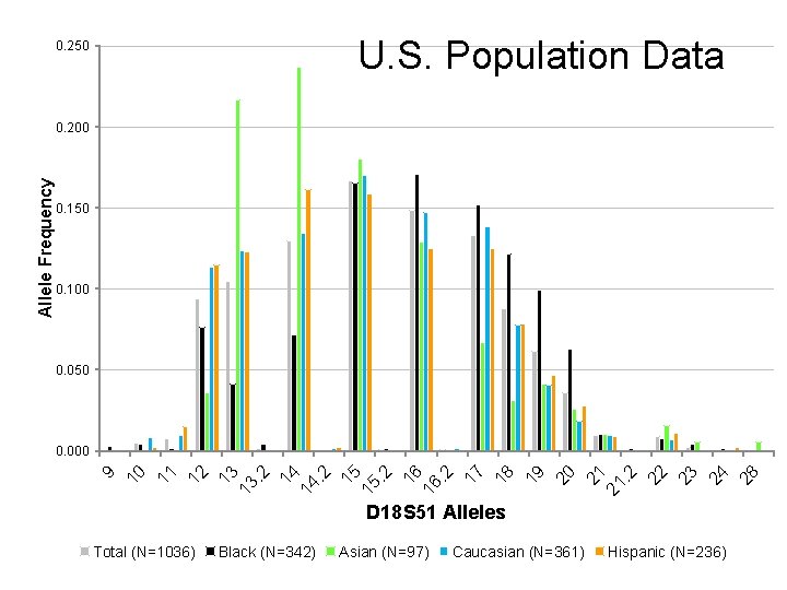
U. S. Population Data 0. 250 0. 100 0. 050 D 18 S 51 Alleles Total (N=1036) Black (N=342) Asian (N=97) Caucasian (N=361) Hispanic (N=236) 28 24 23 22 . 2 21 21 20 19 18 17 . 2 16 16 . 2 15 15 . 2 14 14 . 2 13 13 12 11 10 0. 000 9 Allele Frequency 0. 200

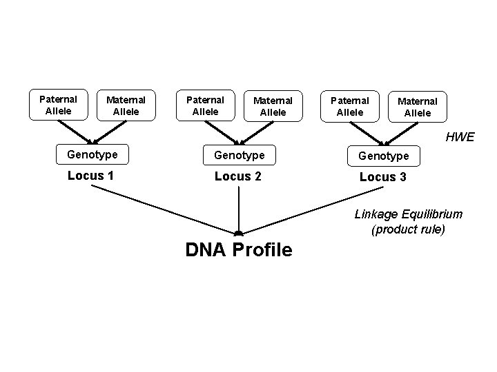
Paternal Allele Maternal Allele HWE Genotype Locus 1 Locus 2 Locus 3 Linkage Equilibrium (product rule) DNA Profile

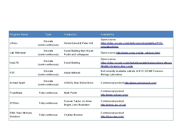
Program Name Type Creator(s) Availability LRmix Discrete (semi-continuous) Hinda Haned & Peter Gill Open-source https: //sites. google. com/site/forensicdnastatistics/PCRsimulation/lrmix Lab Retriever Discrete (semi-continuous) David Balding then Norah Rudin and colleagues Open-source http: //www. scieg. org/lab_retriever. html like. LTD Discrete (semi-continuous) David Balding Open-source https: //sites. google. com/site/baldingstatisticalgenetics/software /likeltd-r-forensic-dna-r-code FST Discrete (semi-continuous) Adele Mitchell Not currently available outside of NYC OCME Forensic Biology Laboratory Armed Xpert Discrete (semi-continuous) USACIL then Niche. Vision Commercial product http: //www. armedxpert. com/ True. Allele Fully-continuous Mark Perlin Commercial product http: //www. cybgen. com/ STRmix Fully-continuous Duncan Taylor, Jo-Anne Bright, John Buckleton Commercial product http: //strmix. esr. cri. nz/ DNA View Mixture Solution Fully-continuous Charles Brenner Commercial product http: //dna-view. com/

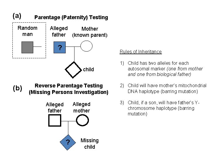
(a) Parentage (Paternity) Testing Random man Alleged Mother father (known parent) ? Rules of Inheritance child (b) Reverse Parentage Testing (Missing Persons Investigation) Alleged mother Alleged father ? Missing child 1) Child has two alleles for each autosomal marker (one from mother and one from biological father) 2) Child will have mother’s mitochondrial DNA haplotype (barring mutation) 3) Child, if a son, will have father’s Ychromosome haplotype (barring mutation)

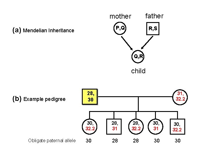
(a) Mendelian Inheritance mother father P, Q R, S Q, R child (b) Example pedigree Obligate paternal allele 28, 30 31, 32. 2 30, 32. 2 28, 31 28, 32. 2 30, 31 30, 32. 2 30 28 28 30 30

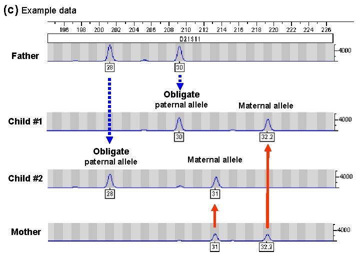
(c) Example data Father Obligate paternal allele Maternal allele Child #1 Obligate paternal allele Child #2 Mother Maternal allele

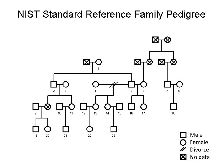
NIST Standard Reference Family Pedigree Male Female Divorce No data

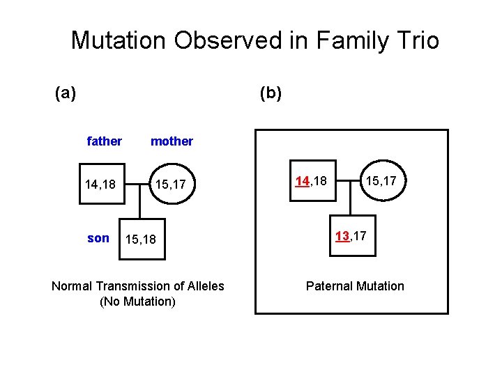
Mutation Observed in Family Trio (a) (b) father 14, 18 son mother 15, 17 15, 18 Normal Transmission of Alleles (No Mutation) 14, 18 15, 17 13, 17 Paternal Mutation

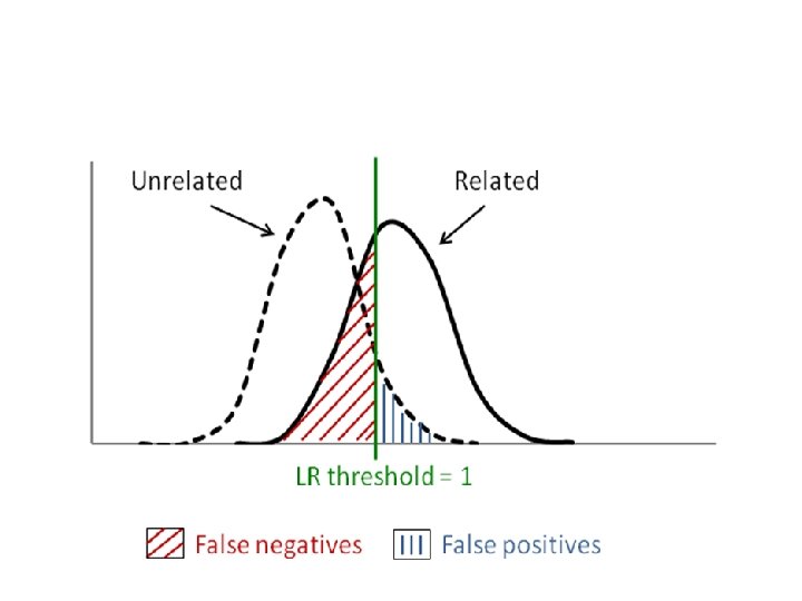
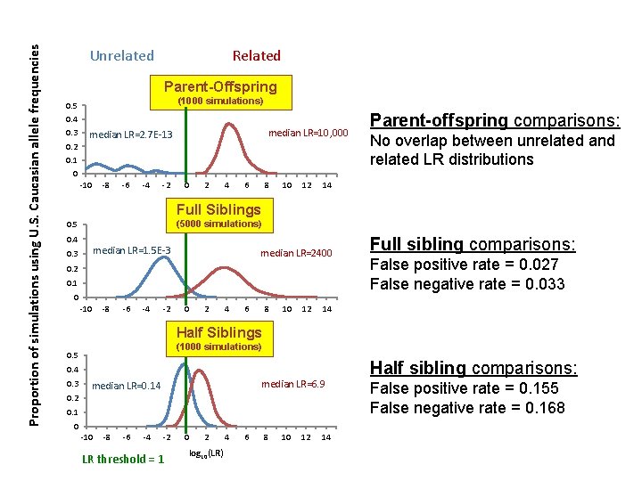
Proportion of simulations using U. S. Caucasian allele frequencies Unrelated Related Parent-Offspring (1000 simulations) 0. 5 0. 4 0. 3 0. 2 median LR=10, 000 median LR=2. 7 E-13 0. 1 0 -10 -8 -6 -4 -2 0 2 4 6 8 10 12 Parent-offspring comparisons: No overlap between unrelated and related LR distributions 14 Full Siblings (5000 simulations) 0. 5 0. 4 median LR=1. 5 E-3 0. 3 median LR=2400 0. 2 0. 1 0 -10 -8 -6 -4 -2 0 2 4 6 8 10 12 Full sibling comparisons: False positive rate = 0. 027 False negative rate = 0. 033 14 Half Siblings (1000 simulations) 0. 5 0. 4 0. 3 median LR=6. 9 median LR=0. 14 0. 2 0. 1 0 -10 -8 -6 -4 -2 LR threshold = 1 0 2 log 10(LR) 4 6 8 10 12 14 Half sibling comparisons: False positive rate = 0. 155 False negative rate = 0. 168

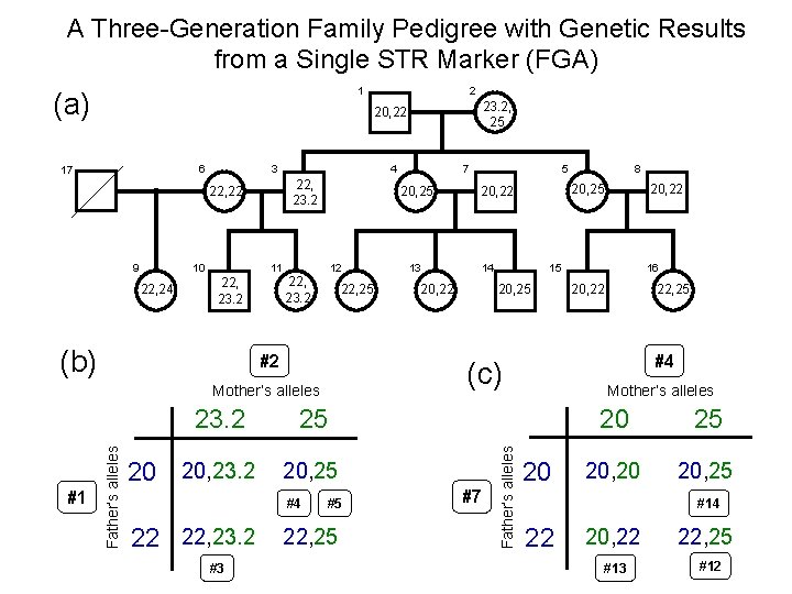
A Three-Generation Family Pedigree with Genetic Results from a Single STR Marker (FGA) 1 (a) 23. 2, 25 20, 22 3 22, 22 9 10 22, 24 11 22, 23. 2 (b) 4 22, 23. 2 20, 25 12 22, 23. 2 22, 25 #2 Father’s alleles 20 20, 23. 2 #3 14 20, 22 #5 22, 25 #7 20, 22 15 20, 25 8 20, 25 20, 22 16 20, 22 22, 25 #4 Mother’s alleles 25 #4 22 22, 23. 2 13 5 (c) Mother’s alleles 23. 2 7 Father’s alleles 6 17 #1 2 20 20 25 20, 20 20, 25 #14 22 20, 22 #13 22, 25 #12

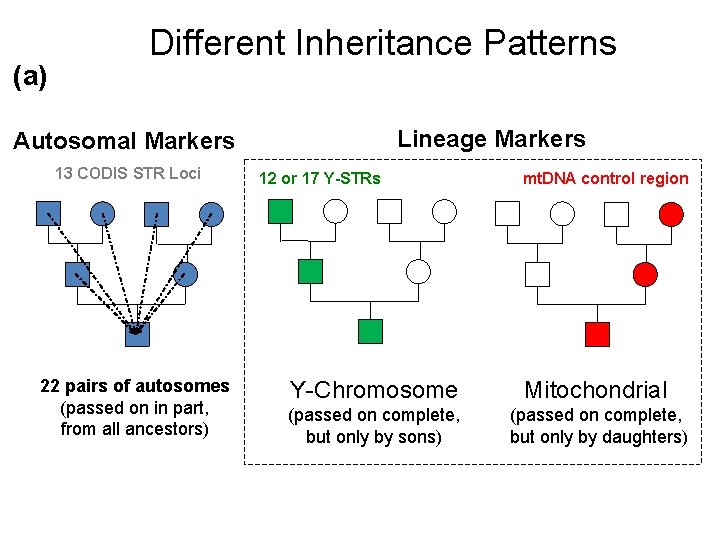
(a) Different Inheritance Patterns Lineage Markers Autosomal Markers 13 CODIS STR Loci 22 pairs of autosomes (passed on in part, from all ancestors) 12 or 17 Y-STRs mt. DNA control region Y-Chromosome Mitochondrial (passed on complete, but only by sons) (passed on complete, but only by daughters)

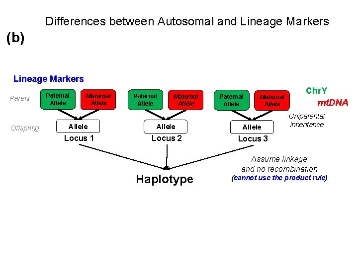
Differences between Autosomal and Lineage Markers (b) Lineage Markers Parent Offspring Paternal Allele Maternal Allele Allele Locus 1 Locus 2 Locus 3 Haplotype Chr. Y mt. DNA Uniparental inheritance Assume linkage and no recombination (cannot use the product rule)

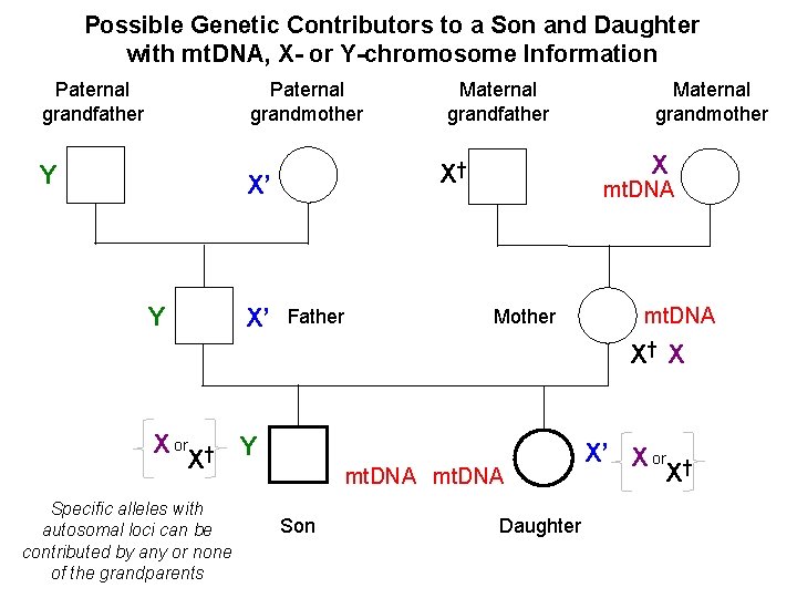
Possible Genetic Contributors to a Son and Daughter with mt. DNA, X- or Y-chromosome Information Paternal grandfather Paternal grandmother Y X’ Father Maternal grandmother X X† X’ Y Maternal grandfather mt. DNA Mother mt. DNA X† X X or † Y X Specific alleles with autosomal loci can be contributed by any or none of the grandparents mt. DNA Son Daughter X’ X or † X

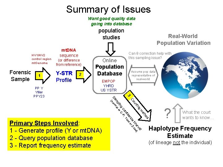
Summary of Issues Want good quality data going into database population studies HV 1/HV 2 control region mt. Genome Forensic Sample 1 (or difference from reference) Y-STR Profile 2 Online Population Database EMPOP YHRD US YSTR Primary Steps Involved: 1 - Generate profile (Y or mt. DNA) 2 - Query population database 3 - Report frequency estimate Can θ correction help with this sampling issue? Assume pop data representative of real-world d ho et m l g va tin er il) un int ta e 2 Co nc l or 3 ide tai nf ; 1 co -P ng r C pli o m al Sa norm ( PP Y Yfiler PPY 23 mt. DNA sequence Real-World Population Variation ? What the court wants to know… Haplotype Frequency Estimate (of lineage not the individual)

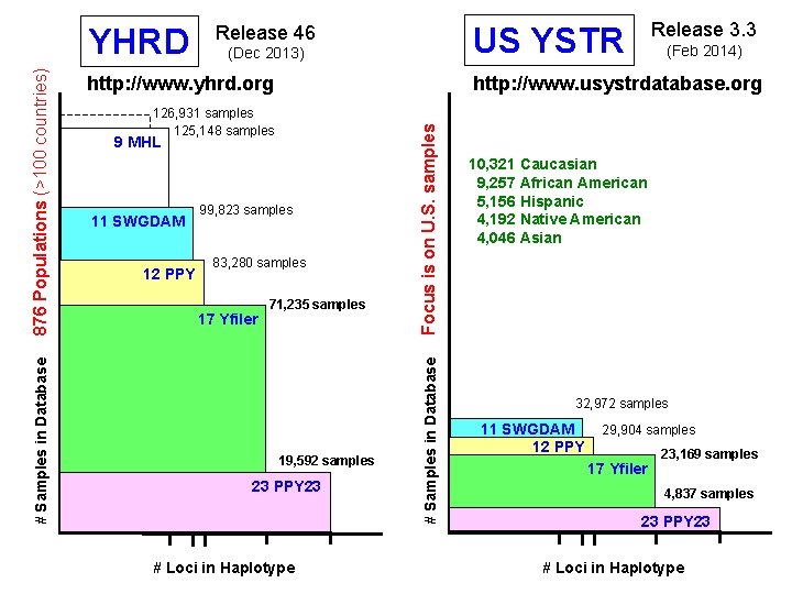
9 MHL 99, 823 samples 83, 280 samples 17 Yfiler 71, 235 samples 19, 592 samples 23 PPY 23 # Loci in Haplotype Focus is on U. S. samples 126, 931 samples 125, 148 samples 12 PPY (Feb 2014) http: //www. usystrdatabase. org http: //www. yhrd. org 11 SWGDAM Release 3. 3 US YSTR (Dec 2013) # Samples in Database 876 Populations (>100 countries) YHRD Release 46 10, 321 Caucasian 9, 257 African American 5, 156 Hispanic 4, 192 Native American 4, 046 Asian 32, 972 samples 11 SWGDAM 12 PPY 29, 904 samples 17 Yfiler 23, 169 samples 4, 837 samples 23 PPY 23 # Loci in Haplotype

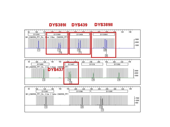
DYS 389 I DYS 437 DYS 439 DYS 389 II

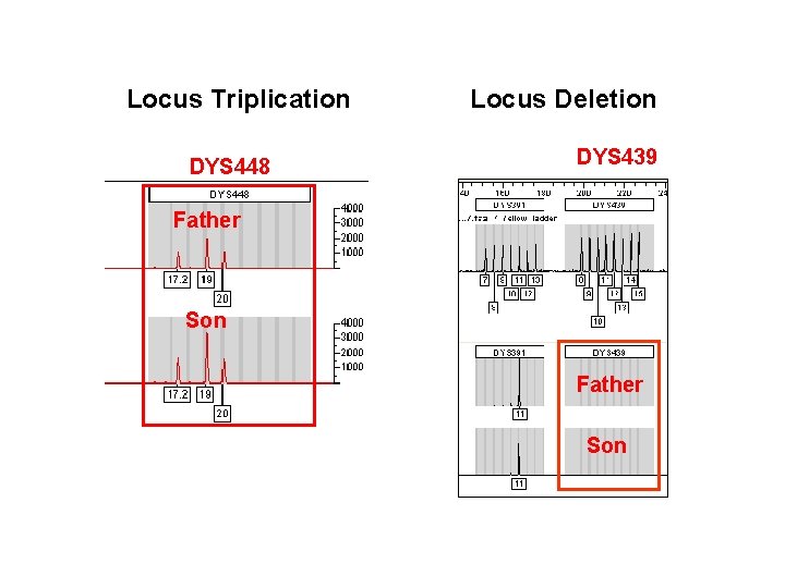
Locus Triplication DYS 448 Locus Deletion DYS 439 Father Son

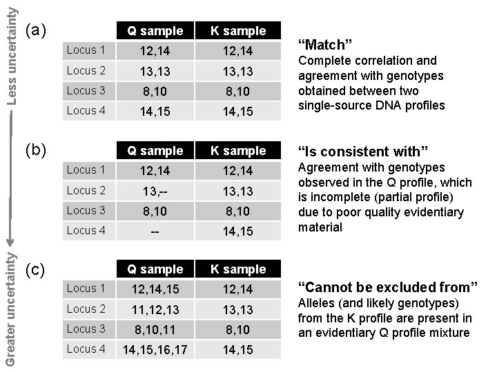
Less uncertainty (a) Q sample K sample Locus 1 12, 14 Locus 2 13, 13 Locus 3 8, 10 Locus 4 14, 15 Q sample K sample Locus 1 12, 14 Locus 2 13, -- 13, 13 Locus 3 8, 10 Locus 4 -- 14, 15 Q sample K sample Locus 1 12, 14, 15 12, 14 Locus 2 11, 12, 13 13, 13 Locus 3 8, 10, 11 8, 10 Locus 4 14, 15, 16, 17 14, 15 Greater uncertainty (b) (c) “Match” Complete correlation and agreement with genotypes obtained between two single-source DNA profiles “Is consistent with” Agreement with genotypes observed in the Q profile, which is incomplete (partial profile) due to poor quality evidentiary material “Cannot be excluded from” Alleles (and likely genotypes) from the K profile are present in an evidentiary Q profile mixture

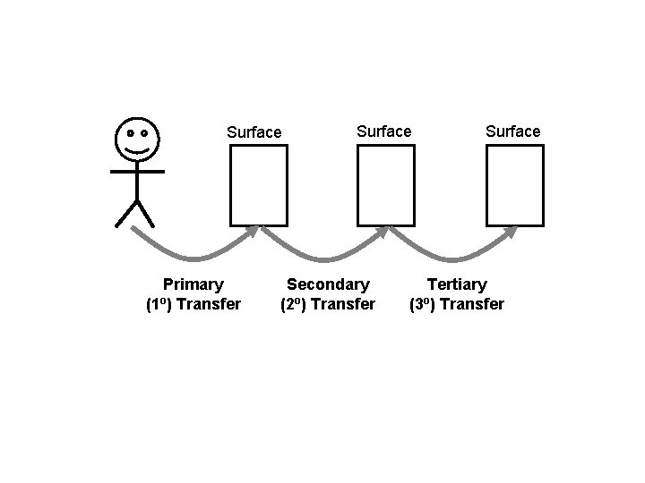
Surface Primary (1 o) Transfer Surface Secondary (2 o) Transfer Surface Tertiary (3 o) Transfer

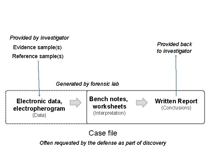
Provided by investigator Provided back to investigator Evidence sample(s) Reference sample(s) Generated by forensic lab Electronic data, electropherogram (Data) Bench notes, worksheets (Interpretation) Written Report (Conclusions) Case file Often requested by the defense as part of discovery

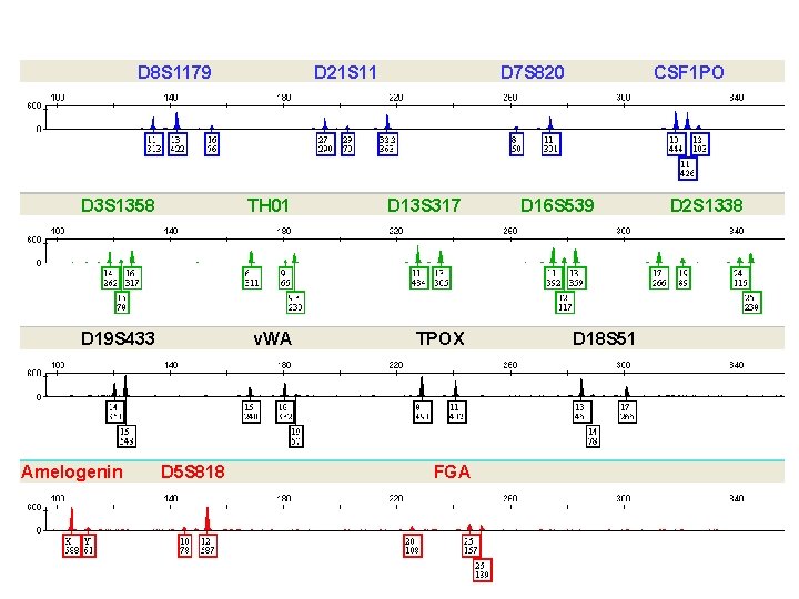
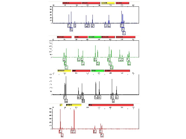
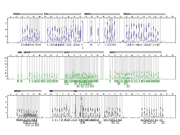
D 8 S 1179 D 21 S 11 D 7 S 820 D 3 S 1358 TH 01 D 13 S 317 D 19 S 433 v. WA TPOX Amelogenin D 5 S 818 FGA CSF 1 PO D 16 S 539 D 18 S 51 D 2 S 1338

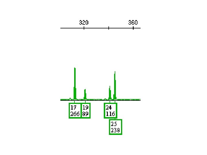
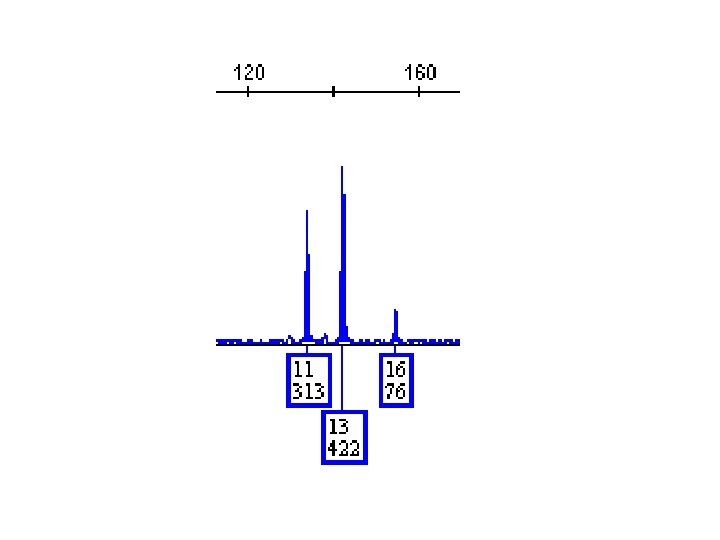
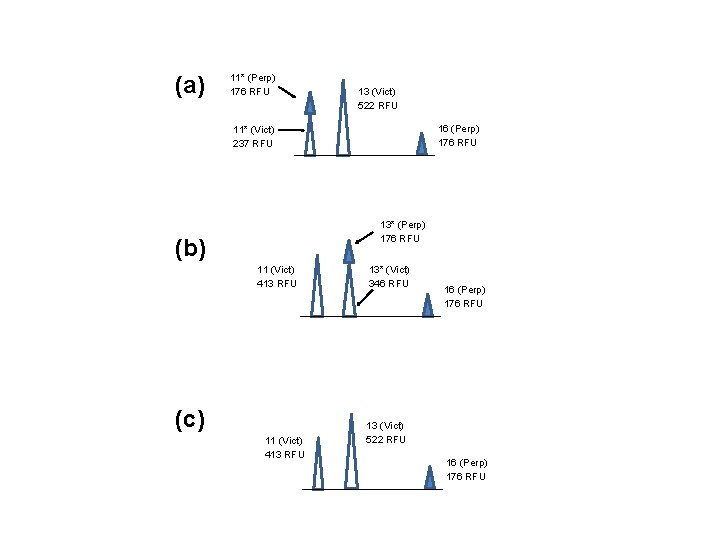
(a) 11* (Perp) 176 RFU 13 (Vict) 522 RFU 16 (Perp) 176 RFU 11* (Vict) 237 RFU 13* (Perp) 176 RFU (b) 11 (Vict) 413 RFU (c) 11 (Vict) 413 RFU 13* (Vict) 346 RFU 16 (Perp) 176 RFU 13 (Vict) 522 RFU 16 (Perp) 176 RFU