PTT 205 By Mrs Noor Amirah Abdul Halim

PTT 205 By: Mrs. Noor Amirah Abdul Halim

� Introduction to Mass Transfer and Diffusions � Molecular Diffusion in Gas � Molecular Diffusion in Liquids � Molecular Diffusion in Biological Materials

May occurs whenever there is a gradient in the concentration of a species. MASS TRANSFER may occur in a gas mixture, a liquid solution or solid The basic mechanisms are the same whether the phase is a gas, liquid, or solid.

Modes of Mass Transfer Diffusion q the net transport of substances in a stationary solid or fluid under a concentration gradient. Advection q the net transport of substances by the moving fluid, and so cannot happen in solids. It does not include transport of substances by simple diffusion. Convection q the net transport of substances caused by both advective transport and diffusive transport (occurs only in fluid)

Diffusion Phenomena

Definition of Concentration i) Number of molecules of each species present per unit volume (molecules/m 3) ii) Molar concentration of species = Number of moles per unit volume (kmol/m 3) iii) Mass concentration = Mass of species per unit volume (kg/m 3)

Mass transfer applications in Chemical/Biological Processes � � � � Distillation Absorption Drying Liquid-liquid extraction Adsorption Ion exchange Crystallization Membrane processes

Fick’s Law for Molecular Diffusion

Diffusivity, (D)

Content: � General molecular diffusion in gas � Case 1 : Equimolar counter diffusion � Case 2 : Diffusion of A and B plus convection � Case 3 : A diffusing through nondiffusing B (stagnant) � Diffusion Coefficient for gases

General Molecular Diffusion in Gas Example 1: Molecular diffusion of Helium in Nitrogen A mixture of He and N 2 gas is contained in a pipe (0. 2 m long) at 298 K and 1 atm total pressure which is constant throughout. The partial pressure of He is 0. 60 atm at one end of the pipe, and it is 0. 20 atm at the other end. Calculate the flux of He at steady state if DAB of He-N 2 mixture is 0. 687 x 10 -4 m 2/s.

Solution: Use Fick’s law of diffusion given by equation (1); Rearranging equation (1) and integrating gives the following: At steady state, diffusion flux is constant. Diffusivity is taken as constant. Therefore, equation (2) gives;

Solution:

Solution: Equation (3) can therefore be written as; Which gives the flux as; Thus,

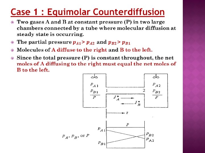
Case 1 : Equimolar Counterdiffusion

Case 1 : Equimolar Counterdiffusion Exercise 1: Ammonia gas (A) is diffusing through a uniform tube 0. 10 m long containing N 2 gas (B) at 1. 0132 x 105 Pa pressure and 298 K. At point 1, p. A 1 = 1. 013 x 104 Pa At point 2, p. A 2 = 0. 507 x 104 Pa. The diffusivity DAB = 0. 230 x 10 -4 m 2/s. (a) Calculate the flux J*A at steady state (b) Repeat for J*B

Case 2 : Diffusion of A and B plus convection � Consider that diffusion of A and B occurs in convective flow where the velocity of diffusion was taken into account. � In previous case only , J*A (diffusive flux-Fick’s Law) is considered due to diffusion occurs in stationary fluid � For diffusion in a convective flow, NA (total flux by convection) is used � Note that flux by convection is consisted of flux by diffusion and flux by advection � Thus the overall flux is a combination of diffusion flux + convection flux

Case 2 : Diffusion of A and B plus convection The simplified equation for diffusion plus convection to use when the flux NA is used: A similar equation can be written for NB

Case 3 : A diffusing through nondiffusing B

Case 3 : A diffusing through nondiffusing B B is nondiffusing, thus NB = 0 The simplified equation to calculate the flux of A in nondiffusing B is given by; A log mean value of inert B is defined as follows:

Case 3 : A diffusing through nondiffusing B Example 2 : Diffusion of water through stagnant, non-diffusing air: Water in the bottom of a narrow metal tube is held at a constant temperature of 293 K. The total pressure of air (assumed to be dry) is 1 atm. Water evaporates and diffuses through the air in the tube, and the diffusion path is 0. 1524 m long. The diffusivity of water vapour at 1 atm and 293 K is 0. 250 x 104 m 2/s. Assume that the vapour pressure of water at 293 K is 0. 0231 atm. Calculate the rate of evaporation at steady state.

Solution: The set-up is shown in the figure. NA = DAB P RT(z 2 – z 1) p. BM Air (B) (p. A 1 - p. A 2 ) 2 where p. BM = (p. A 1 – p. A 2 ) ln[(P - p. A 2 )/ (P - p. A 1 )] z 2 – z 1 Data provided are the following: DAB = 0. 250 x 10 -4 m 2/s; Water (A) P = 1 atm; T = 293 K; z 2 – z 1 = 0. 1524 m; p. A 1 = 0. 0231 atm (saturated vapor pressure); p. A 2 = 0 atm (water vapor is carried away by air at point 2) 1

Solution: Substituting the data provided in the equations given, we get the following:

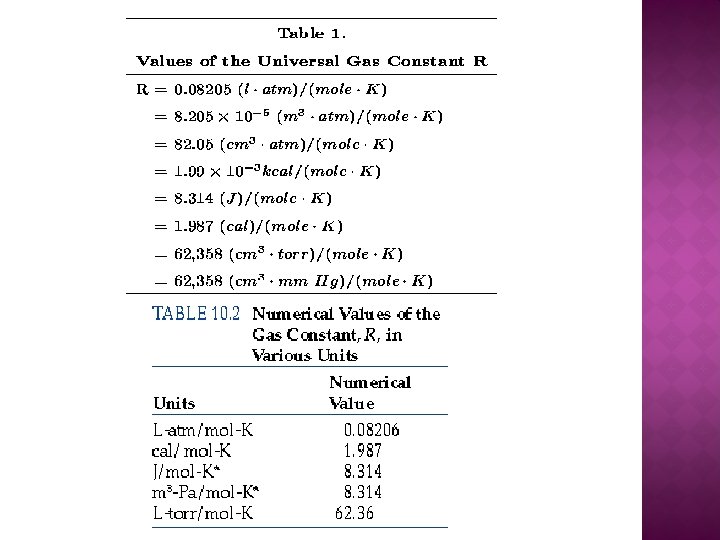
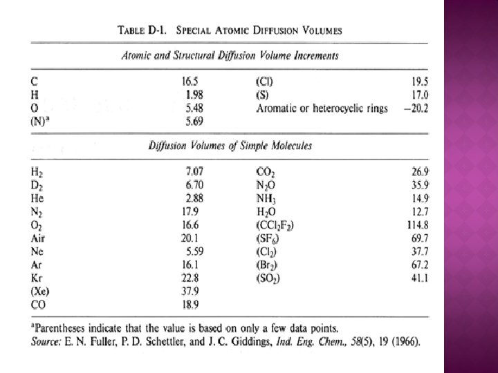
Diffusion Coefficient for Gases

Diffusion Estimation for Gases

Content: � Introduction � Case 1: Equimolar counter diffusion � Case 2: Diffusion of A through nondiffusing B � Diffusion coefficients for liquids � Prediction of diffusivities in liquids

Introduction u Typical phenomena of molecular diffusion in liquids: -liquid extraction -solvent extraction -diffusion of salt in blood u Molecular diffusion in liquid is smaller than molecular diffusion in gases because molecules in liquid are closed together compared to molecules in gas. u Thus, molecules of diffusing solute will collide more frequently with liquid molecules. u Diffusivity in liquid dependent on the concentration of diffusing solute

Case 1: Equimolar counter diffusion

Case 2: Diffusion of A through nondiffusing B

Case 1: Diffusion of A through nondiffusing B Example 3: Diffusion of Ethanol (A) through Water (B) An ethanol (A)-water (B) solution in the form of a stagnant film 2. 0 mm thick at 293 K is in constant at one surface with an organic solvent in which ethanol is soluble and water is insoluble. Hence, NB = 0. At point 1 the concentration of ethanol is 16. 8 wt % and the solution density is ρ1 = 972. 8 kg/m 3. At point 2 the concentration of ethanol is 6. 8 wt % and ρ2 = 988. 1 kg/m 3. The diffusivity of ethanol is 0. 740 x 109 m 2/s. Calculate the steady-state flux, NA.

Solution: Diffusivity, DAB = 0. 740 x 10 -9 m 2/s. Molecular weights of A and B , MA= 46. 05 and MB=18. 02. Mass fraction A at point (2)= 6. 8 wt % Thus, the mole fraction of ethanol (A) is as follows (Assume 100 kg solution: Then XB 2 = 1 -0. 0277 = 0. 9723. Calculating XA 1 = 0. 0732 and XB 1 = 1 -0. 0732 = 0. 9268. To calculate the molecular weight M 2 at point 2,

Solution: Similarly, M 1 = 20. 07. To calculate XBM we can use the linear mean since XB 1 and XB 2 are close to each other: Substituting into equation and solving,

Diffusion coefficients for liquids

Prediction of diffusivities in liquids (Stokes-Einstein Equation)

Prediction of diffusivities in liquids (Wilke-Chang Equation) DAB - diffusivity in m 2/s MB - molecular weight of solvent B T - temperature in K μ - viscosity of solvent B in kg/m s VA - solute molar volume at its normal boiling point in m 3/kmol Φ - association parameter of the solvent, which 2. 6 for water, 1. 9 for methanol, 1. 5 for ethanol, and so on

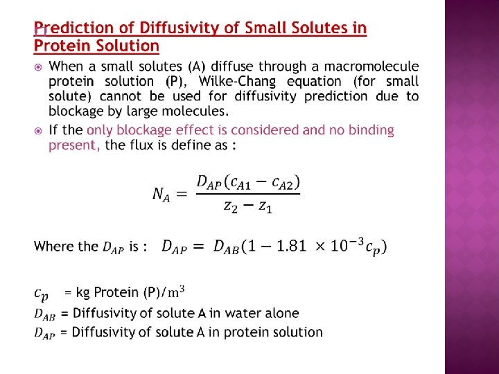
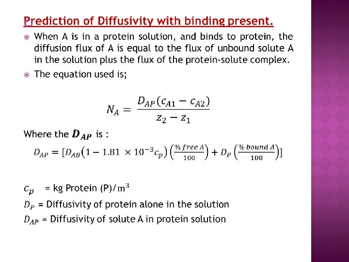
Content: � Diffusion of biological solutes in liquids � Diffusion Coefficient for Biological Solutes in Aqueous Solution � Prediction of Diffusivity for Biological Solutes � Interactions and Binding in Diffusion of Protein Colloids. � Prediction of Diffusivity of Small Solutes in Protein Solution � Prediction of Diffusivity with Binding Present

Diffusion of biological solutes in liquids Example of applications Food Processing � Diffusion of volatile constituents in food materials through the liquid during evaporation Fermentation Process � Diffusion of nutrients, sugar, oxygen to the microorganisms. � Diffusion of waste product and enzyme from microorganisms. Medical Application � Dialysis machine - Diffusion of various waste products from blood to a membrane and through membrane to an aqueous solution

Diffusion Coefficient for Biological Solutes in Aquoues Solution

Prediction of Diffusivity for Biological Solutes Wilke-Chang Equation § § Small solutes in aqueous solution with molecular weight less than 1000 or solute molar less than about 0. 500 m 3/kmol Refer to liquid diffusion part Stokes-Einstein Equation § § For larger solutes Refer to liquid diffusion part Modified Polson Equation § § § For a molecular weight above 1000 MA= MW for large molecule A Suitable for sphere-shaped molecules

Prediction of Diffusivity for Biological Solutes Example 4 : Prediction of diffusivity of Albumin Predict the diffusivity of bovine serum albumin at 298 K in water as a dilute solution using the modified Polson equation and compare with the experimental value in Table 6. 4 -1.

Solution: The molecular weight of bovine serum albumin (A) From Table 6. 4 -1 is MA= 67500 kg/kg mol. The viscosity of water at 25 °C is 0. 8937 x 10 -3 Pa. s at T= 298 K. Substituting into Polson Equation This value is 11% higher than the experimental value of 6. 81 x 10 -11 m 2/s

Interactions and Binding in Diffusion of Protein Colloids. q Macromolecule in solution having large molecular weight were often called as `colloids` q The diffusion behavior of protein colloids in solution is affected by their large size and shapes q Protein colloids have a number of sites for interaction or binding of the solute or ligand molecules. q Thus, diffusion of macromolecules such as protein and small solutes (e. g urea, KCl) can be greatly affected by the presence together of both types of molecules even in dilute solution