Psychology 253 Section 4 Regularized Regression Lecture 1

Psychology 253, Section 4: Regularized Regression, Lecture 1 • Regularized (or penalized, or ridge) regression can be done in R with the functions, lm. ridge {MASS} and glmpath {glmpath} • Examine Alan Gordon’s EEG data (Thanks, Alan, for this gift!), and the {glmpath} data set, ‘heart. data’, both with binary DV’s. Hence we use the generalized linear model for logistic regression. • But before tackling yet another regression package, let us take stock. 1

R packages for regression analyses Ewart Thomas 1. lm {stats}: Quantitative dependent variable (DV), fixed effects OLS model. This workhorse function, the General Linear Model, in the base package accepts quantitative or categorical predictors. 2. glm {stats}: Quantitative DV (including binary DV), fixed effects logistic regression model. This Generalized Linear Model in the base package accepts quantitative or categorical predictors, as well as link functions other than the logistic. 3. lmer {lme 4}: Quantitative DV (including binary DV), mixed effects model; with a choice of link functions. This is an expansion of lm() to handle random effects.

4. mlogit {mlogit}: Categorical DV (or DV is ranking of k options), multinomial logistic regression model, with alternative-specific and/or participant-specific variables, and extensions to random effects. 5. clm/clm 2 {ordinal}: Ordinal DV, cumulative link model (CLM). The latent variable distribution can be Logistic, Normal, etc. , and the cut-points, or thresholds, on the latent variable scale can be estimated. Random effects can be handled by clmm(), using the same syntax as lmer(), and by the older clmm 2(), using the same syntax as lme(). 6. lrm {rms}: Ordinal DV, logistic regression models (LRM) in the package, Regression Modeling Strategies. This gives similar output to clm().

7. glmpath {glmpath}: Quantitative DV (including binary DV), fixed effects regression model, with a penalty on the magnitude of the coefficients, e. g. , on the L 1 - and L 2 -norms. This is a generalized linear model that allows for family = c(‘binomial’, ‘gaussian’, ‘poisson’). Regularization with the L 1 -norm is known by the meaningful acronym, LASSO (Least Absolute Shrinkage & Selection Operator) ; that with a mixture of norms is called an elastic net. 8. lm. ridge {MASS}: Quantitative DV fixed effects regression model, with a penalty on the L 2 -norm of the coefficients. Unlike glmpath(), it handles only Gaussian DV’s (i. e. , it is like lm() not glm()). This is ridge regression, or Tikhonov regularization, and is adequate for many purposes. Now to discuss regularized regression!

EEG Data from Alan Gordon, Ph. D student On May 7, 2012, at 6: 01 PM, Alan Gordon wrote: Hi Ewart, I'm happy to help. Attached is a dataset I use in penalized logistic regression. The question here is: can we use EEG data from the parietal lobe to predict whether people are correctly identifying a stimulus as previously encountered (hits) or correctly identifying a stimulus as not previously encountered (correct rejections). Each EEG feature is a given time bin of amplitude, for a given channel located on the parietal lobe. So, for instance, one feature might be the mean amplitude of channel 45 from time 100 -150 ms after stimulus onset. The data is organized as 254 (memory trials) by 523 (features). The 254 -length label vector is 1 for hits, -1 for correct rejections. For this subject, I can classify at about 65%, where chance is ~50%. Let me know if you'd like more information. I'm happy to see that regularized regression is being discussed in Psy 253! -Alan

Sparse logistic regression for whole brain classification of f. MRI data Srikanth Ryali, 1 Kaustubh Supekar, 2, 3 Daniel A. Abrams, 1 and Vinod Menon Stanford University Neuroimage. 2010 June; 51(2): 752– 764. Multivariate pattern recognition methods are increasingly being used to identify multiregional brain activity patterns that collectively discriminate one cognitive condition or experimental group from another, using f. MRI data. The performance of these methods is often limited because the number of regions considered in the analysis of f. MRI data is large compared to the number of observations (trials or participants). Existing methods that aim to tackle this dimensionality problem are less than optimal because they either over-fit the data or are computationally intractable. Here, we describe a novel method based on logistic regression using a combination of L 1 and L 2 norm regularization that more accurately estimates discriminative brain regions across multiple conditions or groups. The L 1 norm, computed using a fast estimation procedure, ensures a fast, sparse and generalizable solution; the L 2 norm ensures that correlated brain regions are included in the resulting solution, a critical aspect of f. MRI data analysis often overlooked by existing methods. …

Ill-conditioned problems (Wiki) • Hadamard’s (1865 -1963) definition of a well-posed problem: (i) A solution exists. (ii) The solution is unique. And (iii) The solution depends continuously on the data. • If a problem is ill-conditioned (i. e. , not well-posed), it needs to be re-formulated for numerical treatment. Typically this involves including additional assumptions, such as simplicity and smoothness of solution. This process is known as regularization, and Tikhonov regularization, in which the L 2 norm is used, is popular for the regularization of linear ill-conditioned problems. [One approach to data mining. ]

Overdetermined data sets • Suppose we have many fewer observations, yj, j = 1, 2, …, n, than predictor variables, xij, i = 1, 2, …, p; p >> n. We wish to fit the logistic model, • There would be very many solutions, {bi}, and each would yield perfect prediction of the existing data, but poor prediction of new data. • We need to add constraints to the optimization in order to obtain ‘desired’ solutions. These constraints are often on the size (smaller coeffs are preferred), or number (fewer coeffs are preferred, i. e. , parsimony) of the bi.

Estimation goals • Two non-complementary goals. The estimated model should have: – a small error, SSE, in accounting for the observed data – a small error, labeled, e. g. , PRESS (for PREdicted SS), in predicting new data • To calculate PRESS, we can use, say, 90% of the data to estimate a model, use the model to ‘predict’ the remaining 10%, and calculate the prediction errors in this ‘prediction. ’ This approach is called cross-validation (CV), and it is needed to avoid the danger (i. e. , poor prediction) of over-fitting.

We have already considered this example, in which a polynomial predictor with, say, 7 or 8 terms would have a very small SSE, but a ‘large’ PRESS, whereas a linear predictor would have a larger SSE, but a smaller PRESS. We should penalize the polynomial model for having ‘too many’ predictors.

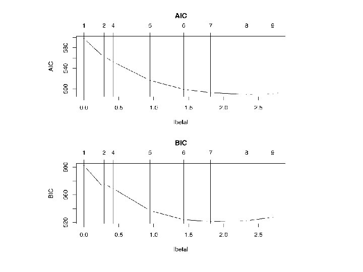
Tradeoff between estimation goals • A tradeoff between SSE and PRESS can occur because, for a given sample size, n, models vary in complexity, defined, say, as p, the number of coefficients, bi. , or in the size (i. e. , the norm) of the coefficients. Increasing the model complexity decreases SSE but increases PRESS. • To manage this tradeoff (i) treat complexity as a ‘cost’ and add it to the error in the data, e. g. , SSE or deviance, to form an overall ‘loss’, J(b), and (ii) find the {bi} that minimizes J(b). A useful index has been the Akaike Information Criterion (AIC), defined as: AIC = deviance + 2(p + 1).

• Let L(y | x, b) be the likelihood, derived from the logistic model, of the data, y, given the predictor matrix, x, and the unknown coefficient vector, b. When using the L 1 -norm, we wish to minimize: • The use of |bi| in the regularization part makes this a non-smooth optimization, because |x| has a ‘kink’ at x = 0. This is the LASSO method.

• The following problems are equivalent: Minimize • When t is very large, the constraint in the 2 nd problem is no longer binding, and we would have unconstrained minimization, just as when λ = 0. Thus small (large) values of λ correspond to large (small) values of t. λ and t are called tuning parameters.

The L 2 -norm • When using the L 2 -norm, we wish to minimize: • The use of bi 2 in the regularization part makes this a smooth optimization known as Tikhonov regularization or ridge regression. • Now we compare the sparseness of solutions under the L 1 -norm and the L 2 -norm.

Sparseness • A solution, {bi}, is said to be sparse if many of the bi ‘s are 0. Sparse solutions are desirable because they help us identify the relevant features for the discrimination reported in y; features with bi = 0 are irrelevant. • As the penalty, λ, increases: (i) under the L 1 norm, some bi do go to 0 and others remain of modest size; whereas (ii) under the L 2 -norm, all bi tend to go to 0. In this way, the L 1 -norm leads to sparse solutions, moreso than the L 2 norm.

Sparseness • Thus choosing the value of λ under the L 1 norm, which results in some bi = 0, is like choosing which predictors to include in a stepwise regression. Cross-validation (CV) is a good tool for estimating the best value for λ. • The criterion used with CV for choosing the best value for λ can be accuracy, AIC, BIC, etc. • However, it is not always true that sparse (i. e. , parsimonious) solutions are most desirable.

Sparseness • Often we wish to know all of the brain regions that are relevant to predicting y. Activity in these relevant regions is likely to be correlated across trials, but the tendency of the LASSO (L 1 -norm) is to select only one of a cluster of intercorrelated regions (it doesn’t care which one), as it generates its sparse solution. • The L 2 -norm is better than the L 1 -norm at selecting groups of correlated predictors.

Elastic nets • The elastic net (Zou & Hastie, 2005) was designed to achieve the sparseness of the LASSO, and the ability of ridge regression to select correlated features. The penalty used is a weighted average of penalties on the L 1 norm and the L 2 -norm. • This model can be rewritten as a type of LASSO and, therefore, can be estimated with the efficiency of the LASSO. • The default in glmpath() is an elastic net with a very small penalty on the L 2 -norm.

The Elastic Net (EN): Minimize: Further improvements are sometimes obtained by inflating the coefficients in this EN solution by a factor, (1 + λ 2).

Regularization and variable selection via the elastic net: by Hui Zou and Trevor Hastie Stanford University, USA. J. R. Statist. Soc. B (2005) 67, Part 2, pp. 301– 320 • “In this paper we propose a new regularization technique which we call the elastic net. Similar to the lasso, the elastic net simultaneously does automatic variable selection and continuous shrinkage, and it can select groups of correlated variables. It is like a stretchable fishing net that retains ‘all the big fish’. Simulation studies and real data examples show that the elastic net often outperforms the lasso in terms of prediction accuracy. ”

‘Why’ the L 1 -norm leads to solutions with ‘many’ bi = 0, i. e. , to sparse solutions As a simple example, consider the cost function, J(b) = b(b/2 – y) + c|b|, c ≥ 0, -Inf < y < Inf. y is the ‘data’, c is the ‘tuning parameter’, and J(0) = 0. We wish to find b* that minimizes J(b). First, suppose c = 0. Then J’(b) = b – y, which is 0 when b = y. Hence J(b) is a minimum when b* = y. Here, the dependence of b* on y is smooth, and b* = 0 only when y = 0. Second, suppose c > 0. The dependence of b* on y is now not smooth.

‘Why’ the L 1 -norm leads to solutions with ‘many’ bi = 0, i. e. , to sparse solutions J(b) b Let J(b) = b(b/2 – y) + c|b|, c > 0, -Inf < y < Inf. We wish to find b* that minimizes J(b). From the plot on the left, we see that, if, as b -> 0 from below, J(b) has a negative slope, and, if, as b -> 0 from above, J(b) has a positive slope, then b* = 0. For this to be true, |y| < c.

The L 1 -norm leads to solutions with ‘many’ bi = 0, i. e. , to sparse solutions J(b) b Let J(b) = b(b/2 – y) + c|b|, c > 0, -Inf < y < Inf. We wish to find b* that minimizes J(b). If y < -c, b* = y + c; If |y| < c, b* = 0; If y > c, b* = y – c. A ‘sparse’ solution, because b* = 0 for a range of y.

Soft Thresholding If y < -c, b* = y + c; If |y| < c, b* = 0; If y > c, b* = y – c These 3 branches of the solution can be described succinctly as: b* = sign(y)(|y| - c)+, which is labeled soft thresholding.

A simple explanation of the Lasso and Least Angle Regression http: //www-stat. stanford. edu/~tibs/lasso/simple. html • Recall Forward Stepwise Regression in the linear model with • – Start with all bi = 0 – Find the predictor, xi 1, most correlated with y, and add it to the model. Compute residuals, r = y – ŷ, which, by definition, are uncorrelated with xi 1. – Continue, at each stage adding to the model the predictor most correlated with r. – Until all predictors are in the model.

A simple explanation of the Lasso and Least Angle Regression http: //www-stat. stanford. edu/~tibs/lasso/simple. html • Forward Stepwise Regression is ‘greedy’ in the sense that it (a) puts ‘all’ of xi 1, the best predictor in the 2 nd stage, into the model, and (b) it ignores useful predictors that happen to have a hi correl with xi 1 and, therefore, a low correl with the residual, r. • Least Angle Regression (LARS, the “S” suggesting “Lasso” and “Stage/Stepwise”) is a less greedy algorithm.

Least Angle Regression (LARS) http: //www-stat. stanford. edu/~tibs/lasso/simple. html • The LARS algorithm (Efron, Hastie, Johnstone & Tibshirani, 2004): – Start with all bi = 0 – Find the predictor, xi 1, most correlated with y, – Increase bi from 0 by a series of small steps in the direction of the sign of its correlation with y. Along the way, compute residuals, r = y – ŷ. Stop when some other predictor, xj 2, has as much correlation with r as xi 1 has. – Increase (bi , bj) in their joint least squares direction until some other predictor, xk, has as much correlation with the residual, r. – Continue until all predictors are in the model. • The LASSO modification: – If a non-zero bi becomes 0, remove it from the active set of predictors and recompute the least-squares direction. This gives the entire path of lasso solutions, as λ and t vary from 0 to Inf.

Psychology 253, Section 4: Regularized Regression, Lecture 2 • Suppose we have many fewer observations, yj, j = 1, 2, …, n, than predictor variables, xij, i = 1, 2, …, p; p >> n). We wish to fit the logistic model, • Many solutions, {bi}, with perfect fit to the existing data, but poor prediction of new data. • We need to add constraints to the optimization in order to obtain ‘desired’ solutions – constraints on the ‘size’ of {bi}. This process is regularization.

More praise for mixed-models Citation: Treating Stimuli as a Random Factor in Social Psychology: A New and Comprehensive Solution to a Pervasive but Largely Ignored Problem. By Judd, Charles M. ; Westfall, Jacob; Kenny, David A. Journal of Personality and Social Psychology, May 21 , 2012,

• … Part of this failure to attend to stimulus variation is due to the demands imposed by traditional analysis of variance procedures for the analysis of data when both participants and stimuli are treated as random factors. In this article, we present a comprehensive solution using mixed models for the analysis of data with crossed random factors (e. g. , participants and stimuli). • We show the substantial biases inherent in analyses that ignore one or the other of the random factors, and we illustrate the substantial advantages of the mixed models approach with both hypothetical and actual, well-known data sets in social psychology …

From an earlier lecture: Crossed random effects • N subjects memorise m faces each under k conditions. Then ‘subno’ and ‘face’ are random effects that are crossed factorially. For each subno*face, we have k repeated measures. rs 1 = lmer(memory ~ condition + (1 | subno) + (1 | face), d) rs 2 = lmer(memory ~ condition + (1 + condition | subno) + (1 | face), d) rs 3 = lmer(memory ~ condition + (1 + condition| subno) + (1 + condition| face), d) • Discuss the assumed random effects! 31

We now return to the lecture on: Types of regularization

LASSO leads to sparse solutions (Good!), but Ridge is better at selecting correlated features. EN is designed to have the benefits of both.

It is helpful to recast these algorithms as ‘minimization subject to a constraint’. (t = ‘radius’ of the lasso!)

glmpath() • glmpath() fits an elastic net: • Its default is a very small penalty, λ 2 = 1 e-05 (i. e. , 10 -5), on the L -norm. So we treat the model as a 2 LASSO and focus on the penalty, λ 1 = λ, on the L 1 norm. • When λ is very large, the regularization term dominates the deviance, and this term [≈ J(b)] is a minimum when Σ|bi| = 0, i. e. , when bi = 0 for all i. As λ is reduced, the first bi to be non-zero will correspond to the feature that correlates most with the response.

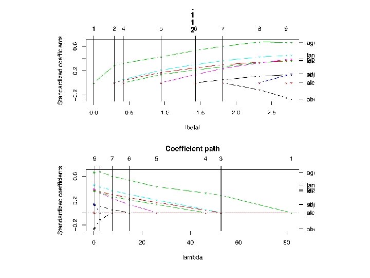
glmpath() • As λ is reduced further, other bi’s become nonzero. In this way, as λ is reduced from a large value to 0, glmpath() keeps track of the path of each bi as it varies from 0 to its value in an unconstrained minimization. • In this way, glmpath() computes “the entire regularization path for generalized linear models with L 1 penalty. ” • The ‘best’ value of λ may be chosen as the value that minimizes AIC or BIC.

An agenda for glmpath() 1. Generate plots of the path of each bi from 0 to its final value, as λ steps from a large value to 0. This is feasible when p ≈ 10, but not when p is ‘large. ’ 2. Plot AIC, BIC for the best model at each λ. And/or print a table with AIC and BIC values. Use these to determine the best value of λ. 3. Which coefficients, bi, are non-zero at the best λ? Does this selection of features lead to any insights about the generation of y? 4. These plots, tables and coefficient sets are produced by glmpath().

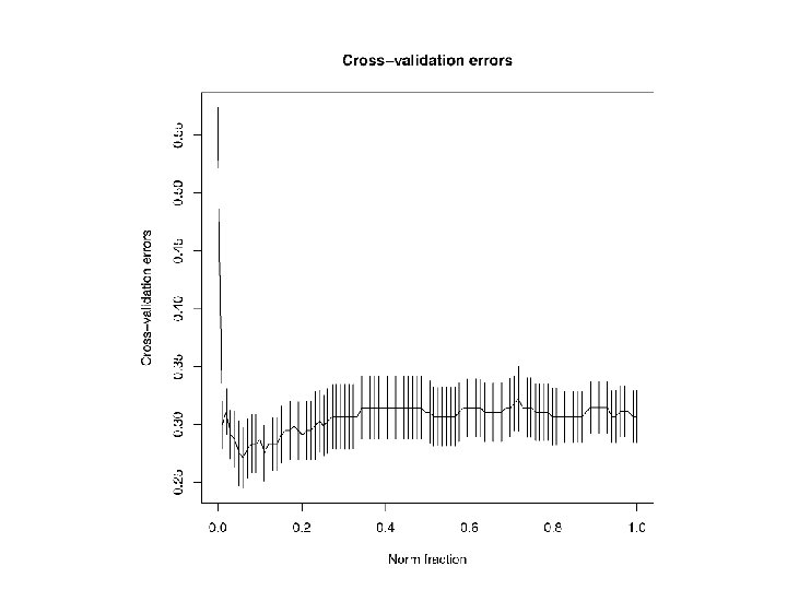
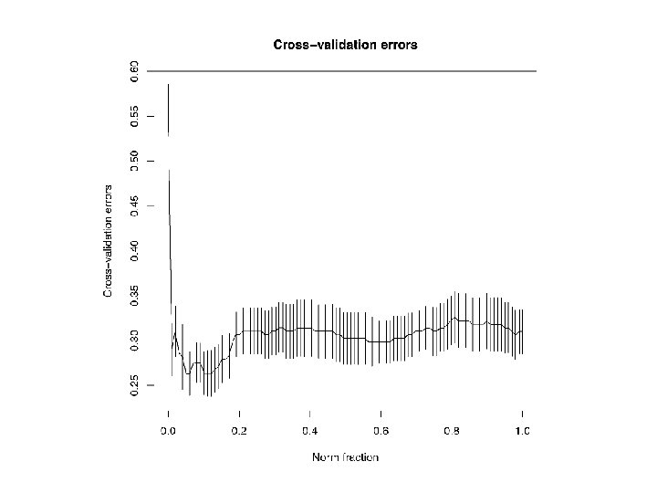
An agenda for glmpath() 5. In addition to AIC and BIC, the cross-validation (CV) accuracy of the best model at each λ can be computed, and the ‘best’ value of λ taken to be the value that maximizes accuracy. 6. The CV plots are produced by cv. glmpath(). 7. Bootstrapping can be used to get the distribution of the coefficients in the best model. For each bi, the histogram can be plotted and the mean and sd can be calculated. 8. These can be done with bootstrap. path() and plot. bootpath().

An agenda for glmpath() 9. If we have independent information about the p features, can this information explain the sign and magnitude of the bi’s? Here, ‘bi’ might be the coefficient estimated from the original data, or the mean of the bootstrapped distribution. Plots and lm() might be applicable here. 10. The default in glmpath() is to set , λ 2 = 1 e-05 (i. e. , 10 -5), as the penalty on the L 2 -norm. Might other values of λ 2 yield even lower AIC or higher CV-accuracy? This can easily be checked.

An agenda for glmpath() 11. If p << n (the ‘normal’ case), how does the LASSO compare with more familiar approaches to model simplification and data condensation, e. g. , • • Stepwise regression PCA or FA on the features; then use factors as predictors of response 12. Empirical studies suggest that no single approach is ‘best’ in ‘most’ situations. Model comparison is always helpful.

glmpath() with Alan’s EEG data • Agenda Items, AI. 1 -AI. 4. In this data set p = 533, so that visualising the path of all the bi’s is not feasible. However, the tables of AIC, BIC, etc. produced by glmpath() suggest that the optimal λ = 0. 028, and the optimal model uses about 107 (about 20%) features, with half of the 107 bi’s positive. • AI. 5 -AI. 6. Cross-validation with cv. glmpath() plots the model performance (CV-accuracy) for the ‘best’ model at each value of λ in seq(0, 1, 100). With Alan’s EEG data, accuracy rates of about 72% are obtained, comparing favorably with the 65% reported earlier. • AI. 7 -AI. 9. Each feature is a known electrode, 1: 13, at a known time bin, 1: 41. So ‘electrode’ and ‘time’ can be used to ‘explain’ bi. • Use smaller data set to fully explore AI. 1 -AI. 11.

library(glmpath) sink('rglmpath 2 a. r’) eeg = read. csv('EEGDat. csv', header=F) eeg = as. matrix(eeg) lab = read. csv('EEGlabels. csv', header=F) lab = as. vector(lab), lab = ifelse(lab == 1, 1, 0) rs 1 = glmpath(eeg, lab, family = binomial) ## With large data set, CV can take 30 mins! ## So I put CV calcs in separate scripts. cv. eeg 1 = cv. glmpath(eeg, lab, family = binomial) #deviance cv. eeg 2 = cv. glmpath(eeg, lab, family = binomial, type='response’) #prediction error

Plot of Lasso coeff vs Time, for each Electrode, 1: 13 Maybe electrodes with |bi| > 10 are relevant?

‘heart. data’ (from {glmpath}) $x sbp tobacco ldl adiposity famhist typea obesity alcohol age 1 160 12. 00 5. 73 23. 11 1 49 25. 30 97. 20 52 2 144 0. 01 4. 41 28. 61 0 55 28. 87 2. 06 63 3 118 0. 08 3. 48 32. 28 1 52 29. 14 3. 81 46 … $y 1 2 3 4 5 6 7 8 9 … 1 1 0 0 1 0 … Predict the presence or absence of heart disease from 9 predictors in S. Africa. x is a matrix, not a dataframe, and y is a vector.

AI. 1 -AI. 4 #glmpath exercises. compare with step() library(glmpath) data(heart. data) attach(heart. data) fit = glmpath(x, y, family = binomial) print(summary(fit)) print(fit$lambda) print(fit$b. predictor) print(fit$actions) detach(heart. data) sink(file=NULL, append=F)

AI. 11 -AI. 12. Comparison with Traditional Stepwise Regression (‘sglmpath 1 b. r’) #glmpath exercises. compare with step() d 0 = data. frame(cbind(x, y)) res 1 = glm(y ~. , family = binomial, d 0) print(summary(res 1)) res 2 = step(res 1) print(summary(res 2))

Results (‘rglmpath 1 b. r’) • Both the familiar lm() (AIC = 492. 14) and the stepwise function, step() (AIC = 487. 69), yield the same ‘best’ set of predictors: tobacco, ldl, famhist, typea, and age. • glmpath() gives a minimum AIC of 489. 27 at Step 10. At Step 9, the active set includes 6 predictors, the above set plus sbp; at Step 10, obesity is added. • The results are similar. • AI. 5 -AI. 9. Predictive accuracy needs to be compared, and bootstrapping used to get the distributions of the coefficients.

Comments on HW-6 • Compare glmpath() with stepwise regression as an automated selection of relevant features, using the self-ratings from HW-3. • Try to explain coefficient values as a function of the ‘loadings’ of the feature (= self-rating) on, say, PC 1 and PC 2. • CV-accuracy: how is this computed?