PSY 6010 Statistics Psychometrics and Research Design Regression

PSY 6010: Statistics, Psychometrics and Research Design Regression (OLS, binary logistic, ordinal) Professor Leora Lawton Spring 2008 Wednesdays 7 -10 PM Room 204 1 1

Regression Steps to conduct a regression analysis 1. 2. 3. 4. 5. 6. 7. 8. Formulate research question Create conceptual model Operationalize Conduct tests on variables Build regression model Run regressions Write up results Interpret results and draw conclusions and/or make recommendations 2 2

1. Formulate Research Question • Understanding the factors behind fertility rates is important because population growth is intrinsic to health, political and economic stability, and the environment. • The debate still rages whether controlling infant mortality is more important in controlling fertility, or whether investing in alternative choices for women provides motivation to lower fertility. In addition, how do different religious groups behave under similar conditions? Moslems have been shown to maintain higher fertility rates despite other signs of modernization. 3 3

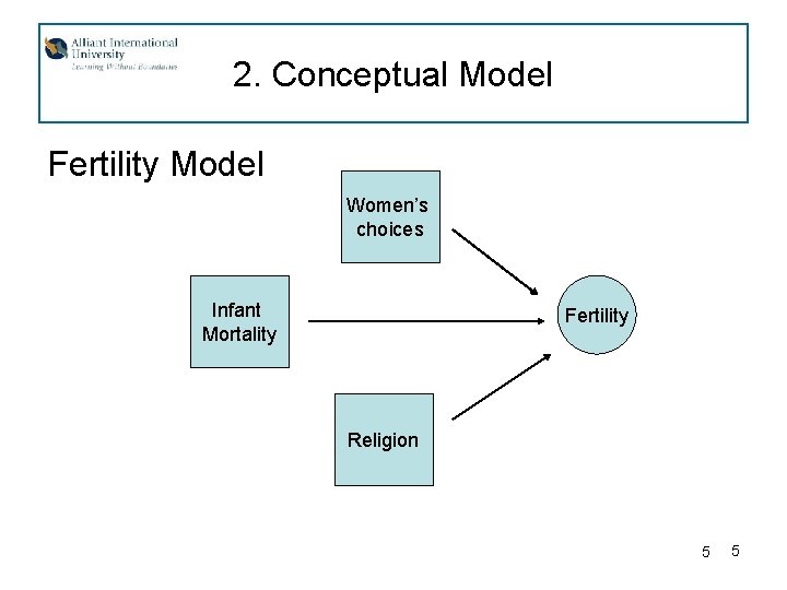
2. Create Conceptual Model • We propose that fertility is higher when infant mortality is higher, because families have ‘replacement children’. • Furthermore, we propose that when women have more choices than family raising, that fertility will be lower. • Finally, we propose that there are religious differences, such that Moslem families will have more children than Christian, Hindu or Buddhist families, because of strong motivations to have ‘what Allah wills’ over alternative religious beliefs of G-d given controls over one’s life path. 4 4

2. Conceptual Model Fertility Model Women’s choices Infant Mortality Fertility Religion 5 5

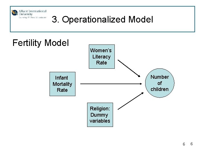
3. Operationalized Model Fertility Model Women’s Literacy Rate Number of children Infant Mortality Rate Religion: Dummy variables 6 6

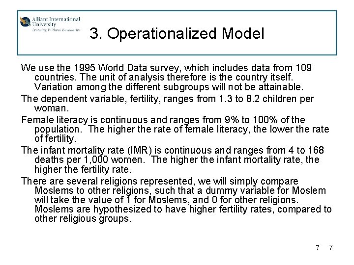
3. Operationalized Model We use the 1995 World Data survey, which includes data from 109 countries. The unit of analysis therefore is the country itself. Variation among the different subgroups will not be attainable. The dependent variable, fertility, ranges from 1. 3 to 8. 2 children per woman. Female literacy is continuous and ranges from 9% to 100% of the population. The higher the rate of female literacy, the lower the rate of fertility. The infant mortality rate (IMR) is continuous and ranges from 4 to 168 deaths per 1, 000 women. The higher the infant mortality rate, the higher the fertility rate. There are several religions represented, we will simply compare Moslems to other religions, such that a dummy variable for Moslem will take the value of 1 for Moslems, and 0 for other religions. Moslems are hypothesized to have higher fertility rates, compared to other religious groups. 7 7

4. Conduct tests on variables • While the initial tests indicate that the independent variables are skewed, we will enter them here as they are. 8 8

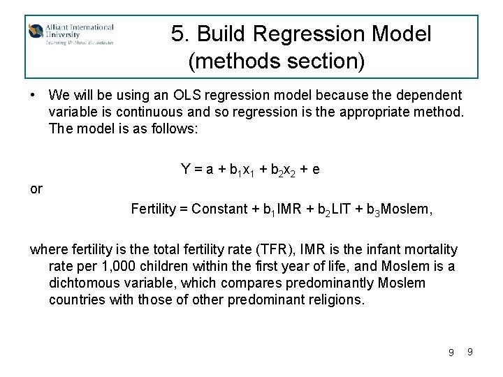
5. Build Regression Model (methods section) • We will be using an OLS regression model because the dependent variable is continuous and so regression is the appropriate method. The model is as follows: Y = a + b 1 x 1 + b 2 x 2 + e or Fertility = Constant + b 1 IMR + b 2 LIT + b 3 Moslem, where fertility is the total fertility rate (TFR), IMR is the infant mortality rate per 1, 000 children within the first year of life, and Moslem is a dichtomous variable, which compares predominantly Moslem countries with those of other predominant religions. 9 9

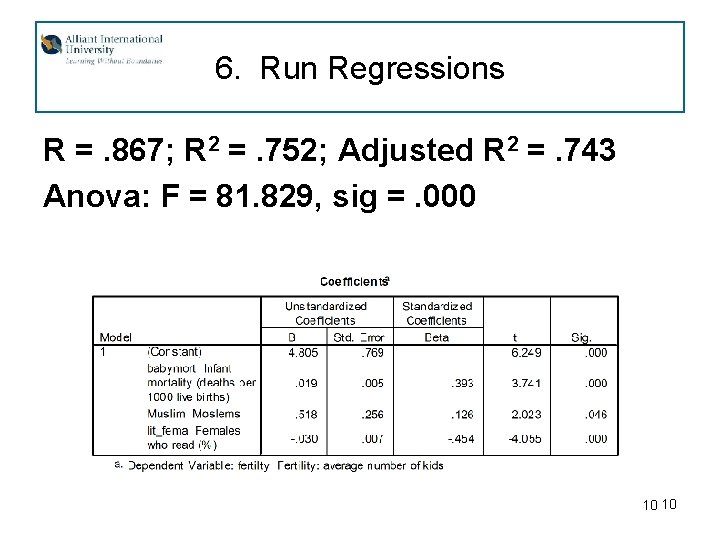
6. Run Regressions R =. 867; R 2 =. 752; Adjusted R 2 =. 743 Anova: F = 81. 829, sig =. 000 10 10

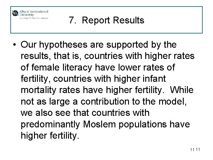
7. Report Results • Our hypotheses are supported by the results, that is, countries with higher rates of female literacy have lower rates of fertility, countries with higher infant mortality rates have higher fertility. While not as large a contribution to the model, we also see that countries with predominantly Moslem populations have higher fertility. 11 11

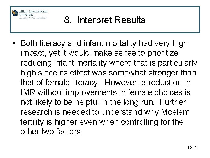
8. Interpret Results • Both literacy and infant mortality had very high impact, yet it would make sense to prioritize reducing infant mortality where that is particularly high since its effect was somewhat stronger than that of female literacy. However, a reduction in IMR without improvements in female choices is not likely to be helpful in the long run. Further research is needed to understand why Moslem fertility is higher even when controlling for the other two factors. 12 12

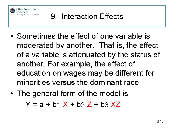
9. Interaction Effects • Sometimes the effect of one variable is moderated by another. That is, the effect of a variable is attenuated by the status of another. For example, the effect of education on wages may be different for minorities versus the dominant race. • The general form of the model is Y = a + b 1 X + b 2 Z + b 3 XZ 13 13

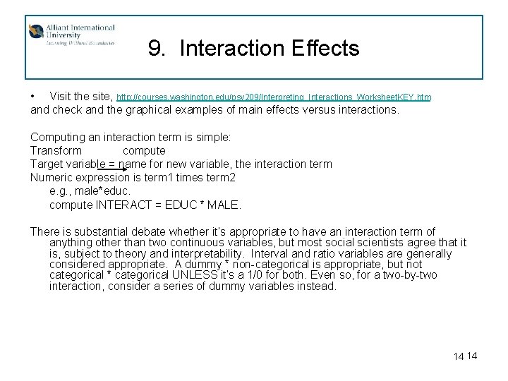
9. Interaction Effects • Visit the site, http: //courses. washington. edu/psy 209/Interpreting_Interactions_Worksheet. KEY. htm and check and the graphical examples of main effects versus interactions. Computing an interaction term is simple: Transform compute Target variable = name for new variable, the interaction term Numeric expression is term 1 times term 2 e. g. , male*educ. compute INTERACT = EDUC * MALE. There is substantial debate whether it’s appropriate to have an interaction term of anything other than two continuous variables, but most social scientists agree that it is, subject to theory and interpretability. Interval and ratio variables are generally considered appropriate. A dummy * non-categorical is appropriate, but not categorical * categorical UNLESS it’s a 1/0 for both. Even so, for a two-by-two interaction, consider a series of dummy variables instead. 14 14

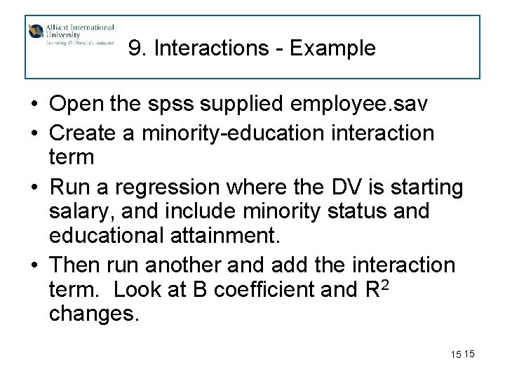
9. Interactions - Example • Open the spss supplied employee. sav • Create a minority-education interaction term • Run a regression where the DV is starting salary, and include minority status and educational attainment. • Then run another and add the interaction term. Look at B coefficient and R 2 changes. 15 15

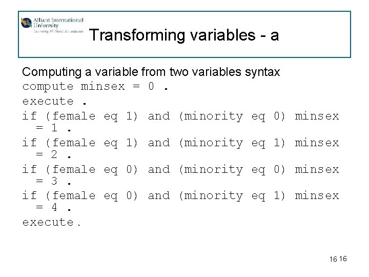
Transforming variables - a Computing a variable from two variables syntax compute minsex = 0. execute. if (female eq 1) and (minority eq 0) = 1. if (female eq 1) and (minority eq 1) = 2. if (female eq 0) and (minority eq 0) = 3. if (female eq 0) and (minority eq 1) = 4. execute. minsex 16 16

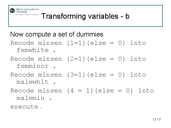
Transforming variables - b Now compute a set of dummies Recode minsex (1=1)(else = femwhite. Recode minsex (2=1)(else = femminor. Recode minsex (3=1)(else = malewhit. Recode minsex (4 = 1)(else malemin. execute. 0) into = 0) into 17 17

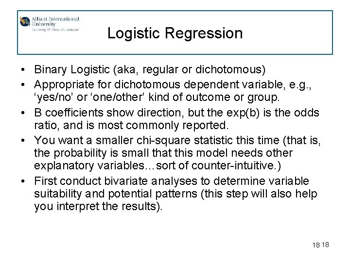
Logistic Regression • Binary Logistic (aka, regular or dichotomous) • Appropriate for dichotomous dependent variable, e. g. , ‘yes/no’ or ‘one/other’ kind of outcome or group. • B coefficients show direction, but the exp(b) is the odds ratio, and is most commonly reported. • You want a smaller chi-square statistic this time (that is, the probability is small that this model needs other explanatory variables…sort of counter-intuitive. ) • First conduct bivariate analyses to determine variable suitability and potential patterns (this step will also help you interpret the results). 18 18

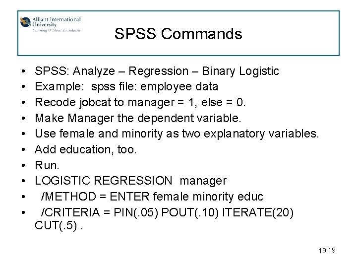
SPSS Commands • • • SPSS: Analyze – Regression – Binary Logistic Example: spss file: employee data Recode jobcat to manager = 1, else = 0. Make Manager the dependent variable. Use female and minority as two explanatory variables. Add education, too. Run. LOGISTIC REGRESSION manager /METHOD = ENTER female minority educ /CRITERIA = PIN(. 05) POUT(. 10) ITERATE(20) CUT(. 5). 19 19

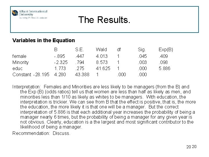
The Results. Variables in the Equation female Minority educ Constant -28. 195 B -. 895 -2. 325 1. 773 4. 280 S. E. . 447. 794. 275 43. 388 Wald 4. 013 8. 573 41. 625 1 df 1 1 1. 000 Sig. . 045. 003. 000 Exp(B). 409. 098 5. 886 Interpretation: Females and Minorities are less likely to be managers (from the B) and the Exp (B) (odds ratios) tell us that women are less than half as likely as men, and minorities less than 1/10 as likely as whites to be managers. With education, the interpretation is trickier. We can see from B that the effect is positive, that is, the more the education, the more likely it is that one will be a manager. But the correct interpretation of 5. 886 is that each additional year increases the probability of being a manager nearly 6 times, but the probability of being a manager for any given year is not obvious. Clearly, education is a the largest and most significant contributor to the likelihood of being a manager. Recommendation: Discuss. 20 20

Ordinal Logistic Regression • Appropriate for a non-continuous but ordinal that is inappropriate for OLS regression (too few categories, or the order is ordered but hard to interpret). • Need to distinguish between IVs that are factors (categorical variables) and covariates (continuous or at least, non-categorical). • Useful to understand predictors of different levels of the DV (analogous to OLS). 21 21

Website Reference for Ordinal and Multinomial Logistic Regression • http: //www. xs 4 all. nl/~jhckx/spss/mlogist/ • Click on the appropriate link: • Example of multinomial logistic regression using NOMREG Example of ordered logistic regression using PLUM 22 22

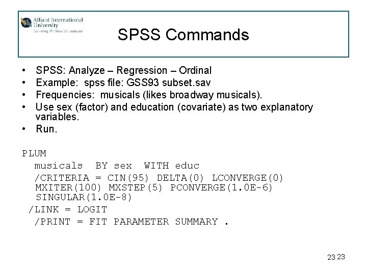
SPSS Commands • • SPSS: Analyze – Regression – Ordinal Example: spss file: GSS 93 subset. sav Frequencies: musicals (likes broadway musicals). Use sex (factor) and education (covariate) as two explanatory variables. • Run. PLUM musicals BY sex WITH educ /CRITERIA = CIN(95) DELTA(0) LCONVERGE(0) MXITER(100) MXSTEP(5) PCONVERGE(1. 0 E-6) SINGULAR(1. 0 E-8) /LINK = LOGIT /PRINT = FIT PARAMETER SUMMARY. 23 23

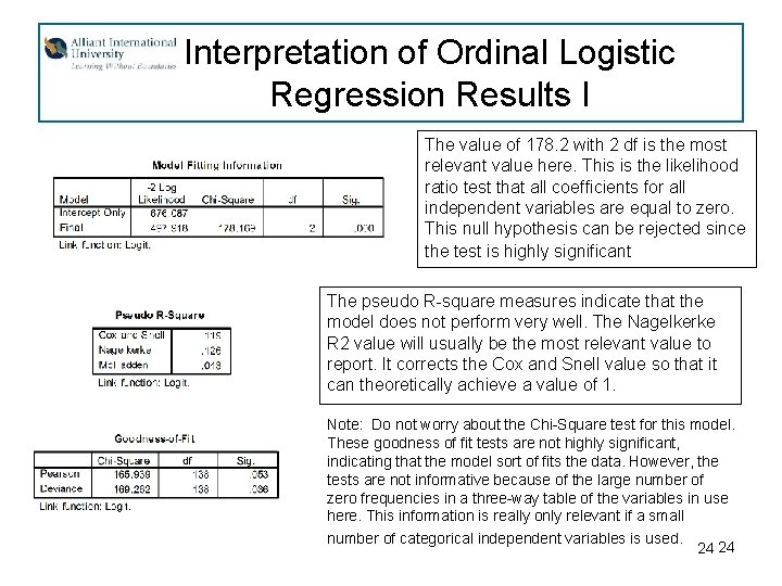
Interpretation of Ordinal Logistic Regression Results I The value of 178. 2 with 2 df is the most relevant value here. This is the likelihood ratio test that all coefficients for all independent variables are equal to zero. This null hypothesis can be rejected since the test is highly significant The pseudo R-square measures indicate that the model does not perform very well. The Nagelkerke R 2 value will usually be the most relevant value to report. It corrects the Cox and Snell value so that it can theoretically achieve a value of 1. Note: Do not worry about the Chi-Square test for this model. These goodness of fit tests are not highly significant, indicating that the model sort of fits the data. However, the tests are not informative because of the large number of zero frequencies in a three-way table of the variables in use here. This information is really only relevant if a small number of categorical independent variables is used. 24 24

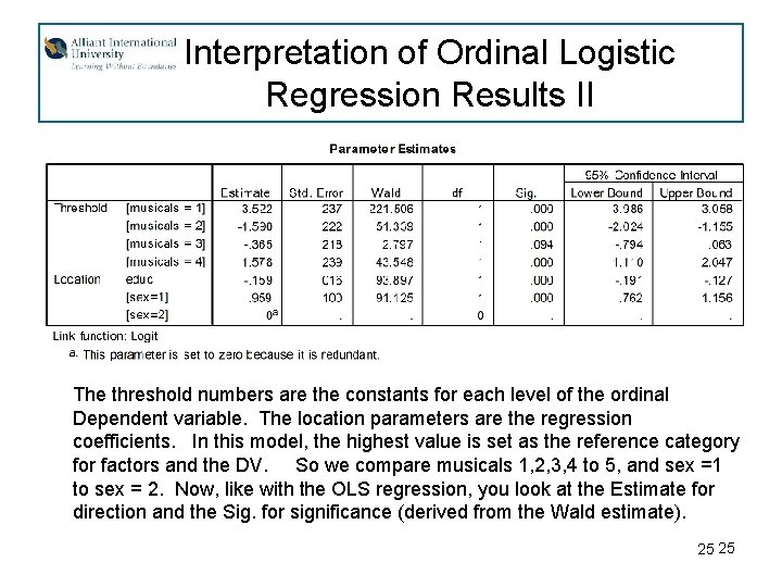
Interpretation of Ordinal Logistic Regression Results II The threshold numbers are the constants for each level of the ordinal Dependent variable. The location parameters are the regression coefficients. In this model, the highest value is set as the reference category for factors and the DV. So we compare musicals 1, 2, 3, 4 to 5, and sex =1 to sex = 2. Now, like with the OLS regression, you look at the Estimate for direction and the Sig. for significance (derived from the Wald estimate). 25 25

Interpretation of Ordinal Logistic Regression Results II • The problem is, right now the interpretation reads the more education one has, the less one is likely to dislike Broadway Musicals, and Sex = 1 (males) are more likely to dislike musicals. This is a bit backwards, so that’s why it’s good to reverse the coding on the DV, and also clarify the coding on the IV dummies (from SEX to MALE. You know how to do the dummies, here’s how to do the switch in codes for a numeric variable: • Go to Transform – Automatic Recode • Add in the variable you want to transform, and give it a new name (so you leave the original variable alone) • Click on Recode Starting from the HIGHEST Value. OK. • Check your values for the original and transformed to make sure it came out right. 26 26

Multinomial Logistic Regression • Appropriate for a 3 - or maybe 4 -category dependent variable. • Need to distinguish between IVs that are factors (categorical variables) and covariates (continuous or at least, noncategorical). • Useful to predict membership, or alternatively, to understand what kind of people can be found in that group. 27 27

SPSS Commands • SPSS: Analyze – Regression – Multinomial • Example: spss file: GSS 93 subset. sav • Frequencies: wkstat 28 28

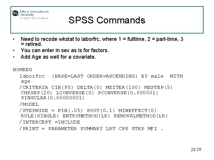
SPSS Commands • • • Need to recode wkstat to laborfrc, where 1 = fulltime, 2 = part-time, 3 = retired. You can enter in sex as is for factors. Add Age as well for a covariate. NOMREG laborfrc (BASE=LAST ORDER=ASCENDING) BY male WITH age /CRITERIA CIN(95) DELTA(0) MXITER(100) MXSTEP(5) CHKSEP(20) LCONVERGE(0) PCONVERGE(0. 000001) SINGULAR(0. 00000001) /MODEL /STEPWISE = PIN(. 05) POUT(0. 1) MINEFFECT(0) RULE(SINGLE) ENTRYMETHOD(LR) REMOVALMETHOD(LR) /INTERCEPT =INCLUDE /PRINT = PARAMETER SUMMARY LRT CPS STEP MFI. 29 29

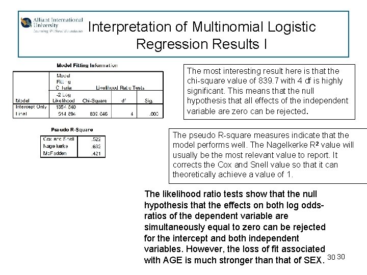
Interpretation of Multinomial Logistic Regression Results I The most interesting result here is that the chi-square value of 839. 7 with 4 df is highly significant. This means that the null hypothesis that all effects of the independent variable are zero can be rejected. The pseudo R-square measures indicate that the model performs well. The Nagelkerke R 2 value will usually be the most relevant value to report. It corrects the Cox and Snell value so that it can theoretically achieve a value of 1. The likelihood ratio tests show that the null hypothesis that the effects on both log oddsratios of the dependent variable are simultaneously equal to zero can be rejected for the intercept and both independent variables. However, the loss of fit associated with AGE is much stronger than that of SEX. 30 30

Interpretation of Multinomial Logistic Regression Results II 31 31

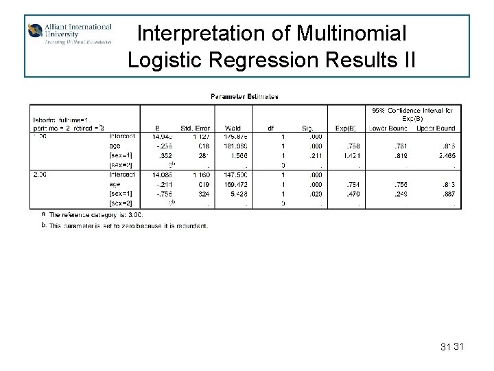
Interpretation of Multinomial Logistic Regression Results II • Interpretation of Multinomial Logistic Regression One category chosen as reference group • odds of being in category other than reference • • Now, this one is like the dichotomous logistic regression, we’re back with the Exp(B) coefficient (Exp(B) is the Odds Ratio). Now we see the odds ratio at any category of marital status on the first two categories of labor force, as compared to the third category. For age, the older you get the less likely you are to be working full or part time compared to being retired (but let’s look at the compare means). For the factors (categorical independent variables), you can enter them without transformation. Males are more likely to be in the fulltime labor force compared to retired than are women, and less likely to be parttime than retired compared to women. 32 32

Crosstabs Sex and Labor Force 33 33