PSF Modeling using Double Zernikes and Nodal Aberration

PSF Modeling using Double Zernikes and Nodal Aberration Theory Insights Brian Bauman Lawrence Livermore National Laboratory LSST 2018 Project & Community Workshop August 15, 2018 #lsst 2018 LSST Project and Community Workshop 2018 • Tucson • August 13 - 17 1

Approach - Create model of telescope aberrations using Double Zernike polynomials (DZ’s) - Misalignments included with small number of DZ’s, informed by Nodal Aberration Theory - For a given field point, we can generate the wavefront - Apply vignetting model - Calculate PSF #lsst 2018 LSST Project and Community Workshop 2018 • Tucson • August 13 - 17 2

Nodal Aberration Theory - Nodal Aberration Theory describes what happens to the aberrations of an optical system when optics are decentered/tilted - Analytic, quantitative #lsst 2018 LSST Project and Community Workshop 2018 • Tucson • August 13 - 17 3

Nodal Aberration Theory - Surfaces contribute aberration fields • • spherical aberration (constant with field) coma (linear with field) astigmatism (quadratic with field) field curvature (quadratic with field) - When these surfaces are decentered/tilted, they produce aberrations that have a lower-order dependence in field #lsst 2018 LSST Project and Community Workshop 2018 • Tucson • August 13 - 17 4

Nodal Aberration Theory - Surfaces contribute aberration fields • • spherical aberration (constant with field) no change coma (linear with field) coma (constant with field) astigmatism (quadratic with field) astig (linear, const w/field) field curvature (defocus, quadratic with field) field tilt, defocus - When these surfaces are decentered/tilted, they produce aberrations that have a lower-order dependence in field - These decentered aberrations are easily calculated - Effects of decenters on higher-order aberrations are often LSST Project and Community Workshop 2018 • Tucson • August 13 - 17 #lsst 2018 negligible 5

Double Zernikes #lsst 2018 LSST Project and Community Workshop 2018 • Tucson • August 13 - 17 6

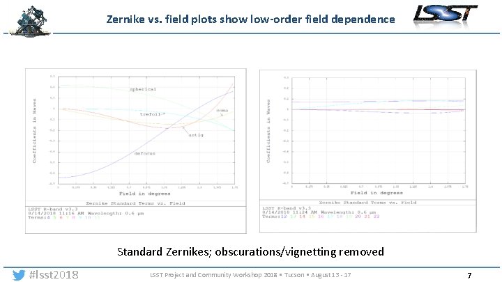
Zernike vs. field plots show low-order field dependence Standard Zernikes; obscurations/vignetting removed #lsst 2018 LSST Project and Community Workshop 2018 • Tucson • August 13 - 17 7

Zernike polynomials - Zernike polynomials are orthonormal over the unit circle, usually pupil #lsst 2018 LSST Project and Community Workshop 2018 • Tucson • August 13 - 17 8

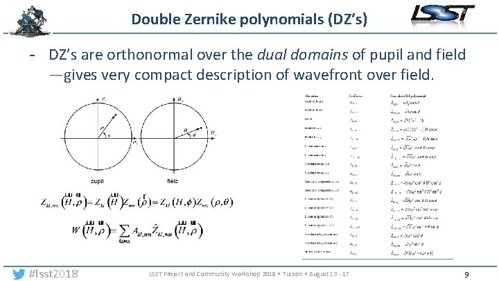
Double Zernike polynomials (DZ’s) - DZ’s are orthonormal over the dual domains of pupil and field —gives very compact description of wavefront over field. #lsst 2018 LSST Project and Community Workshop 2018 • Tucson • August 13 - 17 9

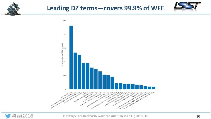
Leading DZ terms—covers 99. 9% of WFE #lsst 2018 LSST Project and Community Workshop 2018 • Tucson • August 13 - 17 10

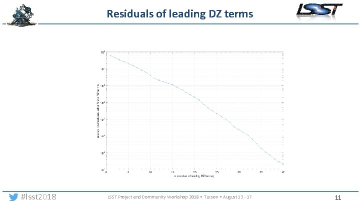
Residuals of leading DZ terms #lsst 2018 LSST Project and Community Workshop 2018 • Tucson • August 13 - 17 11

Rigid-body misalignments - Rigid body misalignments of optics result in just 3 DZ terms: field tilt, linear astigmatism, constant coma - Compensation is performed by secondary decenter/tilt (mostly redundant) and camera hexapod decenter and tilt - Compensators also produce the same 3 DZ terms of field tilt, linear astigmatism, and constant coma - 3 compensators for 3 DZ terms => #lsst 2018 LSST Project and Community Workshop 2018 • Tucson • August 13 - 17 12

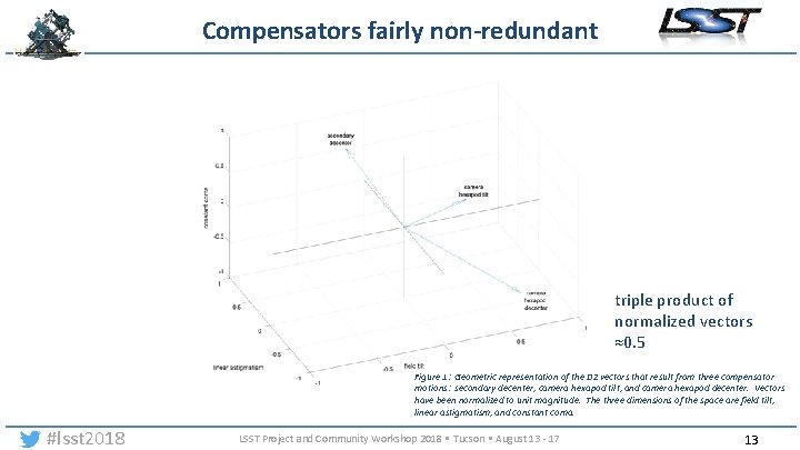
Compensators fairly non-redundant triple product of normalized vectors ≈0. 5 Figure 1: Geometric representation of the DZ vectors that result from three compensator motions: secondary decenter, camera hexapod tilt, and camera hexapod decenter. Vectors have been normalized to unit magnitude. The three dimensions of the space are field tilt, linear astigmatism, and constant coma. #lsst 2018 LSST Project and Community Workshop 2018 • Tucson • August 13 - 17 13

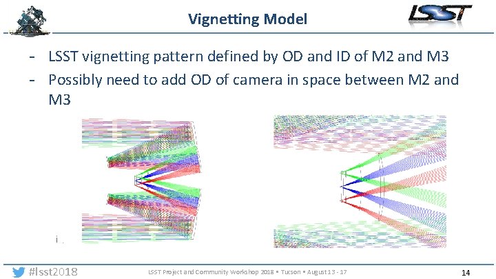
Vignetting Model - LSST vignetting pattern defined by OD and ID of M 2 and M 3 - Possibly need to add OD of camera in space between M 2 and M 3 #lsst 2018 LSST Project and Community Workshop 2018 • Tucson • August 13 - 17 14

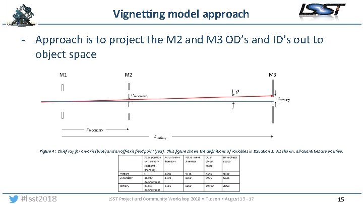
Vignetting model approach - Approach is to project the M 2 and M 3 OD’s and ID’s out to object space Figure 4: Chief ray for on-axis (blue) and an off-axis field point (red). This figure shows the definitions of variables in Equation 1. As shown, all quantities are positive. #lsst 2018 LSST Project and Community Workshop 2018 • Tucson • August 13 - 17 15

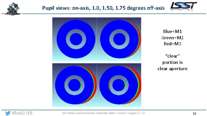
Pupil views: on-axis, 1. 0, 1. 50, 1. 75 degrees off-axis Blue=M 1 Green=M 2 Red=M 3 “clear” portion is clear aperture #lsst 2018 LSST Project and Community Workshop 2018 • Tucson • August 13 - 17 16

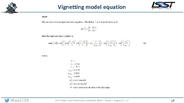
Vignetting model equation #lsst 2018 LSST Project and Community Workshop 2018 • Tucson • August 13 - 17 17

Upcoming work - Chromatic contributions #lsst 2018 LSST Project and Community Workshop 2018 • Tucson • August 13 - 17 18

#lsst 2018 LSST Project and Community Workshop 2018 • Tucson • August 13 - 17 19

#lsst 2018 LSST Project and Community Workshop 2018 • Tucson • August 13 - 17 20

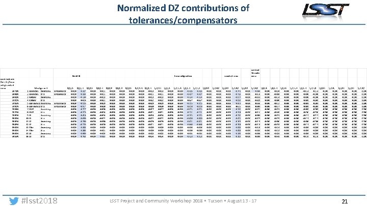
Normalized DZ contributions of tolerances/compensators #lsst 2018 LSST Project and Community Workshop 2018 • Tucson • August 13 - 17 21