Protein structures Protein Structure Why protein structure The

Protein structures

Protein Structure • • Why protein structure? The basics of protein Basic measurements for protein structure Levels of protein structure Prediction of protein structure from sequence Finding similarities between protein structures Classification of protein structures

Why protein structure? • • • In the factory of living cells, proteins are the workers, performing a variety of biological tasks. Each protein has a particular 3 -D structure that determines its function. Protein structure is more conserved than protein sequence, and more closely related to function.

Structural information • Protein Data Bank: maintained by the Research Collaboratory of Structural Bioinformatics(RCSB) • http: //www. rcsb. org/pdb/ > 42752 protein structures as of April 10 • including structures of Protein/Nucleic Acid Complexes, Nucleic Acids, Carbohydrates Most structures are determined by X-ray crystallography. Other methods are NMR and electron microscopy(EM). Theoretically predicted structures were removed from PDB a few years ago. • •

PDB Growth Red: Total Blue: Yearly

The basics of proteins • • Proteins are linear heteropolymers: one or more polypeptide chains Building blocks: 20 types of amino acids. Range from a few 10 s-1000 s Three-dimensional shapes (“fold”) adopted vary enormously.

Common structure of Amino Acid

Formation of polypeptide chain

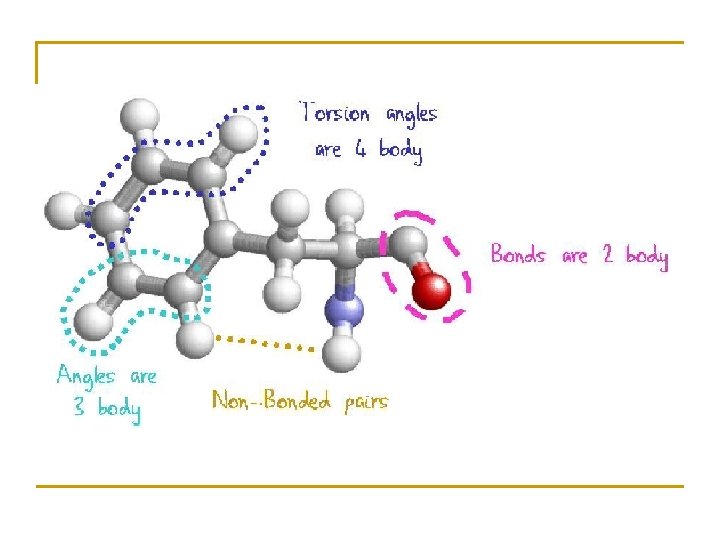
Basic Measurements for protein structure • • • Bond lengths Bond angles Dihedral (torsion) angles

Bond Length • • The distance between bonded atoms is constant Depends on the “type” of the bond Varies from 1. 0 Å(C-H) to 1. 5 Å(C-C) BOND LENGTH IS A FUNCTION OF THE POSITIONS OF TWO ATOMS.

Bond Length

Bond Angles • • All bond angles are determined by chemical makeup of the atoms involved, and are constant. Depends on the type of atom, and number of electrons available for bonding. Ranges from 100° to 180° BOND ANGLES IS A FUNCTION OF THE POSITION OF THREE ATOMS.

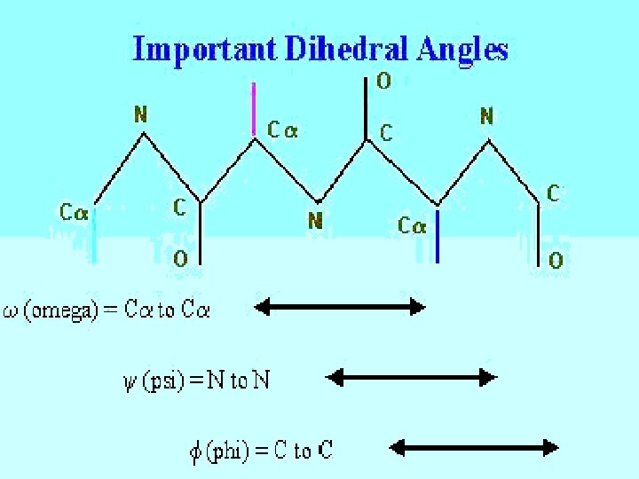
Dihedral Angles • • These are usually variable Range from 0 -360° in molecules Most famous are , , and DIHEDRAL ANGLES ARE A FUNCTION OF THE POSITION OF FOUR ATOMS.

Ramachandran plot

Levels of protein structure • • Primary structure Secondary structure Tertiary structure Quaternary structure

Primary structure • This is simply the amino acid sequences of polypeptides chains (proteins).

Secondary structure • Local organization of protein backbone: -helix, -strand (groups of -strands assemble into -sheet), turn and interconnecting loop. an -helix various representations and orientations of a two stranded b-sheet.

The -helix • One of the most closely packed arrangement of residues. • Turn: 3. 6 residues • Pitch: 5. 4 Å/turn

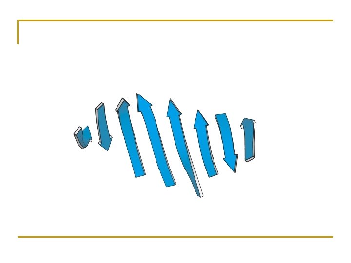
The -sheet • Backbone almost fully extended, loosely packed arrangement of residues.

Anti-parallel beta sheet

Parallel beta sheet

-Sheet (parallel) All strands run in the same direction Catechol O-Methyltransferase

-Sheet (antiparallel) Urate oxidase All strands run in the opposite direction, more stable

Loops and Turns Loops: often contain hydrophilic residue on the surface of proteins Turns: loops with less than 5 residues and often contain G, P

Tertiary structure • • • Description of the type and location of SSEs is a chain’s secondary structure. Three-dimensional coordinates of the atoms of a chain is its tertiary structure. Quaternary structure: describes the spatial packing of several folded polypeptides

Tertiary structure • Packing the secondary structure elements into a compact spatial unit • “Fold” or domain– this is the level to which structure prediction is currently possible.

Quaternary structure • Assembly of homo or heteromeric protein chains. • Usually the functional unit of a protein, especially for enzymes

• Primary and secondary structure are ONEdimensional; Tertiary and quaternary structure are THREE-dimensional. • “structure” usually refers to 3 -D structure of protein.

PDB Files: the “header” HEADER COMPND OURCE AUTHOR REVDAT JRNL JRNL REMARK REMARK REMARK OXIDOREDUCTASE(SUPEROXIDE ACCEPTOR) 13 -JUL-94 MANGANESE SUPEROXIDE DISMUTASE (E. C. 1. 15. 1. 1) COMPLEXED 2 WITH AZIDE (THERMUS THERMOPHILUS, HB 8) M. S. LAH, M. DIXON, K. A. PATTRIDGE, W. C. STALLINGS, J. A. FEE, 2 M. L. LUDWIG 2 15 -MAY-95 1 15 -OCT-94 AUTH M. S. LAH, M. DIXON, K. A. PATTRIDGE, W. C. STALLINGS, AUTH 2 J. A. FEE, M. L. LUDWIG TITL STRUCTURE-FUNCTION IN E. COLI IRON SUPEROXIDE TITL 2 DISMUTASE: COMPARISONS WITH THE MANGANESE ENZYME TITL 3 FROM T. THERMOPHILUS REF TO BE PUBLISHED 1 AUTH M. L. LUDWIG, A. L. METZGER, K. A. PATTRIDGE, W. C. STALLINGS 1 TITL MANGANESE SUPEROXIDE DISMUTASE FROM THERMUS 1 TITL 2 THERMOPHILUS. A STRUCTURAL MODEL REFINED AT 1. 8 1 TITL 3 ANGSTROMS RESOLUTION 1 REF J. MOL. BIOL. V. 219 335 1991 1 REFN ASTM JMOBAK UK ISSN 0022 -2836 1 REFERENCE 2 1 AUTH W. C. STALLINGS, C. BULL, J. A. FEE, M. S. LAH, M. L. LUDWIG 1 TITL IRON AND MANGANESE SUPEROXIDE DISMUTASES: 1 TITL 2 CATALYTIC INFERENCES FROM THE STRUCTURES

PDB Files: the coordinates Atom & Residue ATOM ATOM ATOM ATOM ATOM ATOM 1 2 3 4 5 6 7 8 9 10 11 12 13 14 15 16 17 18 19 20 21 N CA C O CB CG CD 1 CD 2 CE 1 CE 2 CZ OH N CA PRO PRO TYR TYR TYR PRO A A A A A A 1 1 1 1 2 2 2 3 3 XYZ Coordinates 10. 846 12. 063 12. 061 11. 151 12. 010 11. 044 9. 997 13. 050 13. 197 12. 083 11. 733 14. 579 14. 905 14. 516 15. 610 14. 813 15. 924 15. 515 15. 857 11. 583 11. 912 26. 225 25. 940 26. 809 27. 612 24. 474 23. 902 25. 028 26. 576 27. 328 27. 050 25. 895 26. 999 27. 662 27. 092 28. 864 27. 696 29. 465 28. 863 29. 417 28. 094 29. 520 -13. 938 -14. 715 -15. 946 -16. 176 -15. 162 -14. 231 -14. 008 -16. 777 -17. 983 -19. 032 -19. 264 -18. 523 -19. 832 -21. 038 -19. 875 -22. 233 -21. 070 -22. 251 -23. 448 -19. 731 -19. 665 1. 00 1. 00 30. 15 28. 55 26. 17 30. 21 31. 38 31. 86 23. 36 22. 11 21. 02 21. 68 20. 16 19. 42 18. 28 19. 69 19. 13 19. 25 21. 67 19. 90 18. 36 1 MNG 1 MNG 1 MNG 1 MNG 1 MNG 1 MNG 192 193 194 195 196 197 198 199 200 201 202 203 204 205 206 207 208 209 210 211 212

Motifs Helix-loop-helix Four helix bundle Coiled coil

Secondary structure prediction Given a protein sequence (primary structure) • GHWIATR SSECPFIP HWIAT GQLIREAYEDYRHF GQLIREAYEDY SS l Predict its secondary structure content (C=coils H=Alpha Helix E=Beta Strands) CEEEEEC HHCCCCCC EEEEE HHHHHHCCC HHHHHH HH

Why Secondary Structure Prediction? § § § Easier problem than 3 D structure prediction (more than 40 years of history). Accurate secondary structure prediction can be an important information for the tertiary structure prediction Improving sequence alignment accuracy Protein function prediction Protein classification Predicting structural change

Prediction Methods • • Statistical methods • Chou-Fasman method, GOR I-IV Nearest neighbors • NNSSP, SSPAL Neural network • PHD, Psi-Pred, J-Pred Support vector machine

Assumptions § The entire information forming secondary structure is contained in the primary sequence. § Side groups of residues will determine structure. § Examining windows of 13 - 17 residues is sufficient to predict structure.

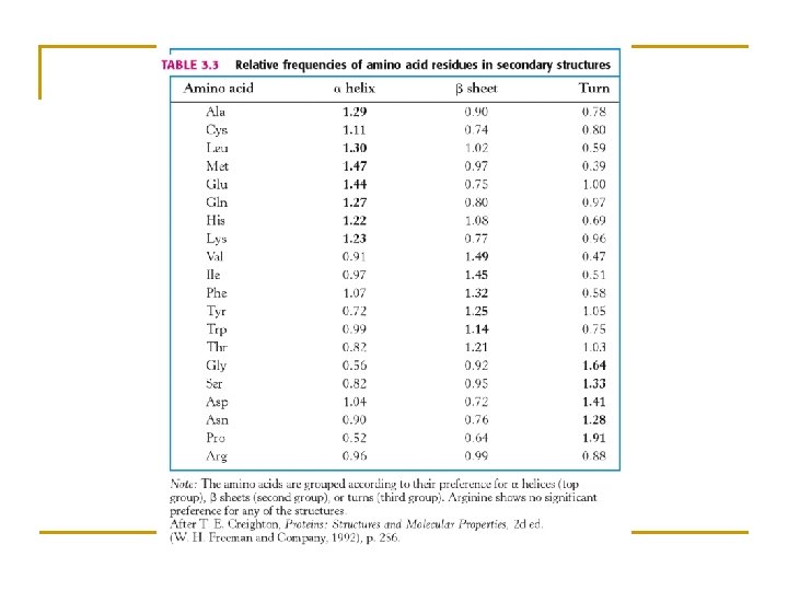
Chou-Fasman method § Compute parameters for amino acids § Preference to be in § alpha helix: P(a) § beta sheet: P(b) § Turn: P(turn) § Frequencies with which the amino acid is in the 1 st, 2 nd, 3 rd, and 4 th position of a turn: f(i), f(i+1), f(i+2), f(i+3). § Use a sliding window

SSE prediction § Alpha-helix prediction § Find all regions where 4 of the 6 amino acids in window have P(a) > 100. § Extend the region in both directions unless 4 consecutive residues have P(a) < 100. § If Σ P(a) > Σ P(b) then the region is predicted to be alpha-helix. § Beta-sheet prediction is analogous. § Turn prediction § Compute P(t) = f(i) + f(i+1) + f(i+2) + f(i+3) for 4 consecutive residues. § Predict a turn if § P(t) > 0. 000075 (check) § The average P(turn) > 100 § Σ P(turn) > Σ P(a) and Σ P(turn) > Σ P(b)

GOR method § Use a sliding window of 17 residues § Compute the frequencies with which each amino acid occupies the 17 positions in helix, sheet, and turn. § Use this to predict the SSE probability of each residue.

Performance of SSE prediction Q 3 and SOV are standards for computing errors A Simple and Fast Secondary Structure Prediction Method using Hidden Neural Networks Kuang Lin, Victor A. Simossis, Willam R. Taylor, Jaap Heringa, Bioinformatics Advance Access published September 17, 2004

Relevance of Protein Structure in the Post-Genome Era structure medicine sequence function

Structure-Function Relationship Certain level of function can be found without structure. But a structure is a key to understand the detailed mechanism. A predicted structure is a powerful tool for function inference. Trp repressor as a function switch

Structure-Based Drug Design Structure-based rational drug design is a major method for drug discovery. HIV protease inhibitor

Experimental techniques for structure determination • X-ray Crystallography • Nuclear Magnetic Resonance spectroscopy (NMR) • Electron Microscopy/Diffraction • Free electron lasers ?

X-ray Crystallography

X-ray Crystallography. . • • From small molecules to viruses Information about the positions of individual atoms Limited information about dynamics Requires crystals

NMR • • Limited to molecules up to ~50 k. Da (good quality up to 30 k. Da) Information about distances between pairs of atoms • • A 2 -d resonance spectrum with offdiagonal peaks Requires soluble, non-aggregating material

Protein Folding Problem A protein folds into a unique 3 D structure under the physiological condition: determine this structure Lysozyme sequence: KVFGRCELAA RGYSLGNWVC QATNRNTDGS RWWCNDGRTP SALLSSDITA DGNGMNAWVA QAWIRGCRL AMKRHGLDNY AAKFESNFNT TDYGILQINS GSRNLCNIPC SVNCAKKIVS WRNRCKGTDV

Levinthal’s paradox • Consider a 100 residue protein. If each residue can take only 3 positions, there are 3100 = 5 1047 possible conformations. • • If it takes 10 -13 s to convert from 1 structure to another, exhaustive search would take 1. 6 1027 years! Folding must proceed by progressive stabilization of intermediates.

Forces driving protein folding • It is believed that hydrophobic collapse is a key driving force for protein folding • • • Hydrophobic core Polar surface interacting with solvent Minimum volume (no cavities) Disulfide bond formation stabilizes Hydrogen bonds Polar and electrostatic interactions

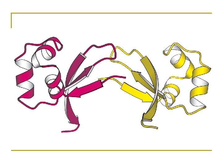
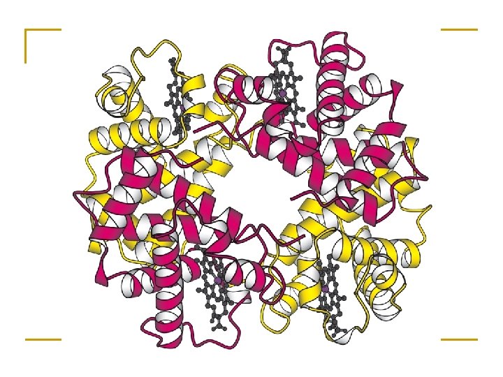
Effect of a single mutation • • Hemoglobin is the protein in red blood cells (erythrocytes) responsible for binding oxygen. The mutation E V in the chain replaces a charged Glu by a hydrophobic Val on the surface of hemoglobin The resulting “sticky patch” causes hemoglobin to agglutinate (stick together) and form fibers which deform the red blood cell and do not carry oxygen efficiently Sickle cell anemia was the first identified molecular disease

Sickle Cell Anemia Sequestering hydrophobic residues in the protein core protects proteins from hydrophobic agglutination.

Protein Structure Prediction • • Ab-initio techniques Homology modeling • • Sequence-sequence comparison Protein threading • Sequence-structure comparison

Lattice models • Simple lattice models (HP-models) • • Two types of residues: hydrophobic and polar 2 -D or 3 -D lattice The only force is hydrophobic collapse Score = number of H H contacts

Scoring Lattice Models • H/P model scoring: count hydrophobic interactions. Score = 5 • Sometimes: • Penalize for buried polar or surface hydrophobic residues

What can we do with lattice models? • • NP-complete For smaller polypeptides, exhaustive search can be used • • Looking at the “best” fold, even in such a simple model, can teach us interesting things about the protein folding process For larger chains, other optimization and search methods must be used • • • Greedy, branch and bound Evolutionary computing, simulated annealing Graph theoretical methods

Representing a lattice model • Absolute directions • • Relative directions • • UURRDLDRRU LFRFRRLLFL Advantage, we can’t have UD or RL in absolute Only three directions: LRF What about bumps? LFRRR • Give bad score to any configuration that has bumps

More realistic models • • Higher resolution lattices (45° lattice, etc. ) Off-lattice models • • Local moves Optimization/search methods and / representations • • • Greedy search Branch and bound EC, Monte Carlo, simulated annealing, etc.

Energy functions An energy function to describe the protein • • • bond energy bond angle energy dihedral angel energy van der Waals energy electrostatic energy Minimize the function and obtain the structure. Not practical in general • • Computationally too expensive Accuracy is poor Empirical force fields • • • Start with a database Look at neighboring residues – similar to known protein folds?

Difficulties Why is structure prediction and especially ab initio calculations hard? • Many degrees of freedom / residue. Computationally too expensive for realistic-sized proteins. • Remote non-covalent interactions • Nature does not go through all conformations • Folding assisted by enzymes & chaperones

Protein Structure Prediction • • Ab-initio techniques Homology modeling • • Sequence-sequence comparison Protein threading • Sequence-structure comparison

Homology modeling steps 1. 2. 3. 4. 5. 6. Identify a set of template proteins (with known structures) related to the target protein. This is based on sequence homology (BLAST, FASTA) with sequence identity of 30% or more. Align the target sequence with the template proteins. This is based on multiple alignment (CLUSTALW). Identify conserved regions. Build a model of the protein backbone, taking the backbone of the template structures (conserved regions) as a model. Model the loops. In regions with gaps, use a loopmodeling procedure to substitute segments of appropriate length. Add sidechains to the model backbone. Evaluate and optimize entire structure.

Homology Modeling • Servers • • SWISS-MODEL ESy. Pred 3 D

Protein Structure Prediction • • • Ab-initio techniques Homology modeling Protein threading • Sequence-structure comparison

Protein threading Structure is better conserved than sequence Structure can adopt a wide range of mutations. Physical forces favor certain structures. Number of folds is limited. Currently ~700 Total: 1, 000 ~10, 000 TIM barrel

Protein Threading • Basic premise The number of unique structural (domain) folds in nature is fairly small (possibly a few thousand) • Statistics from Protein Data Bank (~35, 000 structures) 90% of new structures submitted to PDB in the past three years have similar structural folds in PDB

Concept of Threading o o Thread (align or place) a query protein sequence onto a template structure in “optimal” way Good alignment gives approximate backbone structure Query sequence MTYKLILNGKTKGETTTEAVDAATAEKVFQYANDNGVDGEWTYTE Template set

Threading problem • • Threading: Given a sequence, and a fold (template), compute the optimal alignment score between the sequence and the fold. If we can solve the above problem, then • • • Given a sequence, we can try each known fold, and find the best fold that fits this sequence. Because there are only a few thousands folds, we can find the correct fold for the given sequence. Threading is NP-hard.

Components of Threading Template library • • Use structures from DB classification categories (PDB) Scoring function • • Single and pairwise energy terms Alignment • • • Consideration of pairwise terms leads to NP-hardness heuristics Confidence assessment • • Z-score, P-value similar to sequence alignment statistics Improvements • • Local threading, multi-structure threading

Protein Threading • Build a template database – structure database

Protein Threading – energy function MTYKLILNGKTKGETTTEAVDAATAEKVFQYANDNGVDGEWTYTE how preferable to put two particular residues nearby: E_p how well a residue fits a structural environment: E_s alignment gap penalty: E_g total energy: E_p + E_s + E_g find a sequence-structure alignment to minimize the energy function

Assessing Prediction Reliability MTYKLILNGKTKGETTTEAVDAATAEKVFQYANDNGVDGEWTYTE Score = -1500 Score = -720 Score = -1120 Score = -900 Which one is the correct structural fold for the target sequence if any? The one with the highest score ?

Prediction of Protein Structures • Examples – a few good examples actual predicted

Prediction of Protein Structures • Not so good example

Existing Prediction Programs • PROSPECT • • FUGU • • https: //csbl. bmb. uga. edu/protein_pipeline http: //www-cryst. bioc. cam. ac. uk/~fugue/prfsearch. html THREADER • http: //bioinf. cs. ucl. ac. uk/threader/

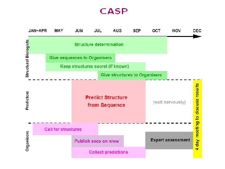
CASP/CAFASP CASP Predictor • CASP: Critical Assessment of Structure Prediction CAFASP Predictor • CAFASP: Critical Assessment of Fully Automated Structure Prediction 1. Won’t get tired 2. High-throughput

CASP 6/CAFASP 4 • • 64 targets Resources for predictors • No X-ray, NMR machines (of course) • CAFASP 4 predictors: no manual intervention • CASP 6 predictors: anything (servers, google, …) Evaluation: • CASP 6 Assessed by experts+computer • CAFASP 4 evaluated by a computer program. • Predicted structures are superimposed on the experimental structures. CASP 7 was held last November

(a) myoglobin (b) hemoglobin (c) lysozyme (d) transfer RNA (e) antibodies (f) viruses (g) actin (h) the nucleosome (i) myosin (j) ribosome Courtesy of David Goodsell, TSRI

Protein structure databases • PDB • • 3 D structures SCOP • • Murzin, Brenner, Hubbard, Chothia Classification • • Class (mostly alpha, mostly beta, alpha/beta (interspersed), alpha+beta (segregated), multi-domain, membrane) Fold (similar structure) Superfamily (homology, distant sequence similarity) Family (homology and close sequence similarity)

The SCOP Database Structural Classification Of Proteins FAMILY: proteins that are >30% similar, or >15% similar and have similar known structure/function SUPERFAMILY: proteins whose families have some sequence and function/structure similarity suggesting a common evolutionary origin COMMON FOLD: superfamilies that have same secondary structures in same arrangement, probably resulting by physics and chemistry CLASS: alpha, beta, alpha–beta, alpha+beta, multidomain

Protein databases • CATH • • • Orengo et al Class (alpha, beta, alpha/beta, few SSEs) Architecture (orientation of SSEs but ignoring connectivity) Topology (orientation and connectivity, based on SSAP = fold of SCOP) Homology (sequence similarity = superfamily of SCOP) • • S level (high sequence similarity = family of SCOP) SSAP alignment tool (dynamic programming)

Protein databases • FSSP • DALI structure alignment tool (distance matrix) • • Holm and Sander MMDB • VAST structure comparison (hierarchical) • Madej, Bryant et al

Protein structure comparison • Levels of structure description • • • Atom/atom group Residue Fragment Secondary structure element (SSE) Basis of comparison • • • Geometry/architecture of coordinates/relative positions sequential order of residues along backbone, . . . physio-chemical properties of residues, …

How to compare? • • • Key problem: find an optimal correspondence between the arrangements of atoms in two molecular structures (say A and B) in order to align them in 3 D Optimality of the alignment is determined using a root mean square measure of the distances between corresponding atoms in the two molecules Complication: It is not known a priori which atom in molecule B corresponds to a given atom in molecule A (the two molecules may not even have the same number of atoms)

Structure Analysis – Basic Issues • Coordinates for representing 3 D structures • • • Cartesian Other (e. g. dihedral angles) Basic operations • • • Translation in 3 D space Rotation in 3 D space Comparing 3 D structures • • • Root mean square distances between points of two molecules are typically used as a measure of how well they are aligned Efficient ways to compute minimal RMSD once correspondences are known (O(n) algorithm) • Using eigenvalue analysis of correlation matrix of points Due to the high computational complexity, practical algorithms rely on heuristics

Structure Analysis – Basic Issues • Sequence order dependent approaches • • • Computationally this is easier Interest in motifs preserving sequence order Sequence order independent approaches • • • More general Active sites may involve non-local AAs Searching with structural information

Find the optimal alignment +

Optimal Alignment • Find the highest number of atoms aligned with the lowest RMSD (Root Mean Squared Deviation) • Find a balance between local regions with very good alignments and overall alignment

Structure Comparison Which atom in structure A corresponds to which atom in structure B ? THESESENTENCESALIGN--NICELY ||| || |||||| THE--SEQUENCE-ALIGNEDNICELY

Structural Alignment An optimal superposition of myoglobin and beta-hemoglobin, which are structural neighbors. However, their sequence homology is only 8. 5%

Structure Comparison Methods to superimpose structures by translation and rotation x 1, y 1, z 1 x 2, y 2, z 2 x 3, y 3, z 3 x 1 + d, y 1, z 1 x 2 + d, y 2, z 2 x 3 + d, y 3, z 3 Translation Rotation

Structure Comparison Scoring system to find optimal alignment Answer: Root Mean Square Deviation (RMSD) n = number of atoms di = distance between 2 corresponding atoms i in 2 structures

Root Mean Square Deviation 3 4 1 5 2 1 2 3 4 5

RMSD Unit of RMSD => e. g. Ångstroms - identical structures => RMSD = “ 0” - similar structures => RMSD is small (1 – 3 Å) - distant structures => RMSD > 3 Å

Pitfalls of RMSD • all atoms are treated equally (e. g. residues on the surface have a higher degree of freedom than those in the core) • best alignment does not always mean minimal RMSD • significance of RMSD is size dependent

Alternative RMSDs • a. RMSD = best root-mean-square distance calculated over all aligned alpha-carbon atoms • b. RMSD = the RMSD over the highest scoring residue pairs • w. RMSD = weighted RMSD Source: W. Taylor(1999), Protein Science, 8: 654 -665.

Structural Alignment Methods • Distance based methods • • • STRUCTAL (Subbiah 1993, Gerstein and Levitt 1996): Dynamic programming to minimize the RMSD between two protein backbones. SSAP (Orengo and Taylor, 1990): Double dynamic programming using intra-molecular distance; CE (Shindyalov and Bourne, 1998): Combinatorial Extension of best matching regions Vector based methods • • • DALI (Holm and Sander, 1993): Aligning 2 -dimensional distance matrices VAST (Madej et al. , 1995): Graph theory based SSE alignment; 3 d. Search (Singh and Brutlag, 1997) and 3 D Lookup (Holm and Sander, 1995): Fast SSE index lookup by geometric hashing. • TOP (Lu, 2000): SSE vector superpositioning. • TOPSCAN (Martin, 2000): Symbolic linear representation of SSE vectors. Both vector and distance based • LOCK (Singh and Brutlag, 1997): Hierarchically uses both secondary structures vectors and atomic distances.

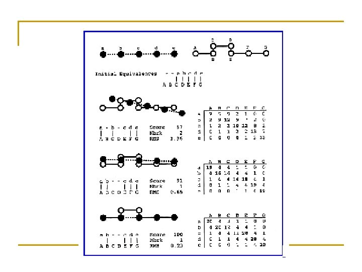
Basic DP (STRUCTAL) 1. 2. 3. 4. Start with arbitrary alignment of the points in two molecules A and B Superimpose in order to minimize RMSD. Compute a structural alignment (SA) matrix where entry (i, j) is the score for the structural similarity between the ith point of A and the jth point of B Use DP to compute the next alignment. Gap cost = 0 5. 6. Iterate steps 2 --4 until the overall score converges Repeat with a number of initial alignments

STRUCTAL • Given 2 Structures (A & B), 2 Basic Comparison Operations 1. Given an alignment optimally SUPERIMPOSE A onto B 2. Find an Alignment between A and B based on their 3 D coordinates Sij = M/[1+(dij/d 0)2] M and d 0 are constants

DALI Method • Distance m. Atrix a. LIgnment • Liisa Holm and Chris Sander, “Protein structure comparison by alignment of distance matrices”, Journal of Molecular Biology Vol. 233, 1993. • Liisa Holm and Chris Sander, “Mapping the protein universe”, Science Vol. 273, 1996. • Liisa Holm and Chris Sander, “Alignment of three-dimensional protein structures: network server for database searching”, Methods in Enzymology Vol. 266, 1996.

How DALI Works? • • Based on fact: similar 3 D structures have similar intra-molecular distances. Background idea • • Represent each protein as a 2 D matrix storing intramolecular distance. Place one matrix on top of another and slide vertically and horizontally – until a common the sub-matrix with the best match is found. Protein A • Protein B Actual implementation • • • Break each matrix into small sub-matrices of fixed size. Pair-up similar sub-matrices (one from each protein). Assemble the sub-matrix pairs to get the overall alignment.

Structure Representation of DALI • 3 D shape is described with a distance matrix which stores all intra-molecular distances between the Cα atoms. • Distance matrix is independent of coordinate frame. • Contains enough information to re-construct the 3 D coordinates. Protein A Distance matrix for Protein A 1 2 3 4 1 0 d 12 d 13 d 14 2 d 12 0 d 23 d 24 3 d 13 d 23 0 d 34 4 d 14 d 24 d 34 0 Distance matrix for 2 drp. A and 1 bbo

Intra-molecular distance for myoglobin

DALI Algorithm 1. Decompose distance matrix into elementary contact patterns (sub-matrices of fixed size) • Use hexapeptide-hexapeptide contact patterns. 2. Compare contact patterns (pair-wise), and store the matching pairs in pair list. 3. Assemble pairs in the correct order to yield the overall alignment.

Assembly of Alignments • Non-trivial combinatory problem. • Assembled in the manner (AB) – (A’B’), (BC) – (B’C’), . . . (i. e. , having one overlapping segment with the previous alignment) • Available Alignment Methods: • Monte Carlo optimization • Brach-and-bound • Neighbor walk

Schematic View of DALI Algorithm 3 D (Spatial) (Sequence) 2 D (Distance Matrix) 1 D

Monte Carlo Optimization • • Used in the earlier versions of DALI. Algorithm • • Compute a similarity score for the current alignment. Make a random trial change to the current alignment (adding a new pair or deleting an existing pair). Compute the change in the score ( S). If S > 0, the move is always accepted. If S <= 0, the move may be accepted by the probability exp(β * S), where β is a parameter. Once a move is accepted, the change in the alignment becomes permanent. This procedure is iterated until there is no further change in the score, i. e. , the system is converged.

Branch-and-bound method • Used in the later versions of DALI. • Based on Lathrop and Smith’s (1996) threading (sequencestructure alignment) algorithm. • Solution space consists of all possible placements of residues in protein A relative to the segment of residues of protein B. • The algorithm recursively split the solution space that yields the highest upper bound of the similarity score until there is a single alignment trace left.

LOCK • • Uses a hierarchical approach Larger secondary structures such as helixes and strands are represented using vectors and dealt with first Atoms are dealt with afterwards Assumes large secondary structures provide most stability and function to a protein, and are most likely to be preserved during evolution

LOCK (Contd. ) • Key algorithm steps: 1. 2. 3. 4. • Represent secondary structures as vectors Obtain initial superposition by computing local alignment of the secondary structure vectors (using dynamic programming) Compute atomic superposition by performing a greedy search to try to minimize root mean square deviation (a RMS distance measure) between pairs of nearest atoms from the two proteins Identify “core” (well aligned) atoms and try to improve their superposition (possibly at the cost of degrading superposition of non-core atoms) Steps 2, 3, and 4 require iteration at each step

Alignment of SSEs • • • Define an orientation-dependent score and an orientationindependent score between SSE vectors. For every pair of query vectors, find all pairs of vectors in database protein that align with a score above a threshold. Two of these vectors must be adjacent. Use orientation independent scores. For each set of four vectors from previous step, find the transformation minimizing rmsd. Apply this transformation to the query. Run dynamic programming using both orientation-dependent and orientation-independent scores to find the best local alignment. Compute and apply the transformation from the best local alignment. Superpose in order to minimize rmsd.

Atomic superposition Loop • • • find matching pairs of C atoms use only those within 3 A find best alignment until rmsd does not change

Core identification Loop • • • find the best core (symmetric nns) and align; remove the rest until rmsd does not change

VAST • • • Begin with a set of nodes (a, x) where SSEs a and x are of the same type Add an edge between (a, x) and (b, y) if angle and distance between (a, b) is same as between (x, y) Find the maximal clique in this graph; this forms the initial SSE alignment Extend the initial alignment to C atoms using Gibbs sampling Report statistics on this match

Quality of a structure match • • • Statistical theory similar to BLAST Compare the likelihood of a match as compared to a random match Less agreement regarding score matrix • z-scores of CE, DALI, and VAST may not be compatible