Protein Structure Prediction Protein Sequence Analysis Molecular properties

Protein Structure Prediction

Protein Sequence Analysis Molecular properties (p. H, mol. wt. isoelectric point, hydrophobicity) Secondary Structure Super-secondary (signal peptide, coiled-coil, transmembrane, etc. ) 3 -D prediction, Threading (tertiary structure) Domains, motifs, etc. Subunit (quaternary structure)

Self-assembly Proteins self-assemble in solution All of the information necessary to determine the complex 3 -D structure is in the amino acid sequences Structure determines function u lock & key model of enzyme function Know the sequence, know the function? Nearly infinite complexity

Structure of Peptide N-terminal C-terminal Peptide Backbone: C’-N-Cα-C’; Dihedral Angle or torsional angle: (Φ, ψ) Instead of 9 variables, use 2 variables (Φ, ψ) for each AA; ω=180 (C’=O and N-H)

Structure prediction Protein Structure prediction is the “Holy Grail” of bioinformatics Since structure = function, then structure prediction should allow protein design, design of inhibitors, etc. Huge amounts of genome data - what are the functions of all of these proteins?

Chemical Properties of Proteins are linear polymers of 20 amino acids Chemical properties of the protein are determined by its amino acids Molecular wt. , p. H, isoelectric point are simple calculations from amino acid composition Hydrophobicity is a property of groups of amino acids - best examined as a graph

(Increase local flexibility) (Increase stability)

Terminology Active site, Blocks, Core, Fold Domain, Motif Family, superfamily Module Class Primary, Secondary, Tertiary, Quaternary

Secondary Structure Protein 2 ndary structure takes one of three forms: uα helix u β sheet u Turn, coil or loop 2 ndary structure are tightly packed in the protein core in a hydrophobic environment 2 ndary structure is predicted within a small window Many different algorithms, not highly accurate Better predictions from a multiple alignment Methods: neural networks, nearest-neighbor method, HMM,

3 -D Structure of Protein Right-hand turn (most), 3. 6 residues per turn, Φ=600, Ψ=400 on average Turn or coil Alpha-helix Antiparallele and parallel Beta-sheet Loop and Turn

Neural Networks for 2 ndary

Protein Structure Classification Class α: a bundle of α helices connected by loops on the surface of protein Class β: antiparallel βsheets Class α/β: mainly parallel βsheets with interveningα helices Class α+β: mainly segregated α helices and antiparallel β sheets Multidomain proteins: comprise domains representing more than one of the above 4 classes Membrane and cell-surface proteins: α helices (hydrophobic) with a particular length range, traversing a membrane

Class β Class α+β Class α/β membrane Membrane proteins

Structure Prediction on the Web Secondary Structural Content Prediction (SSCP): EMBL, Heidelberg n http: //www. bork. embl-heidelberg. de/SSCP/sscp_seq. html BCM Search Launcher: Protein Secondary Structure Prediction: Baylor College of Medicine n http: //dot. imgen. bcm. tmc. edu: 9331/seq-search/struc-predict. html PREDATOR: EMBL, Heidelberg n http: //www. embl-heidelberg. de/cgi/predator_serv. pl UCLA-DOE Protein Fold Recognition Server n http: //www. doe-mbi. ucla. edu/people/fischer/TEST/getsequence. html

“Super-secondary” Structure Common structural motifs n n Membrane spanning Signal peptide Coiled coil Helix-turn-helix

Hydrophobicity Profile for 2 ndary (positions of turns between 2 ndary structure, exposed and buried residues, membranespanning segments, antigenic sites)

3 -D Structure Cannot be accurately predicted from sequence alone (known as ab initio) Levinthal’s paradox: a 100 aa protein has 3200 possible backbone configurations - many orders of magnitude beyond the capacity of the fastest computers There are perhaps only a few hundred basic structures, but we don’t yet have this vocabulary or the ability to recognize variants on a theme Methods: HMM, structure profile method, contact potential method, threading method, conformational energy (monte Carlo Algorithm)

Procedure of Prediction sequence Database similarity search Align Known structure No Family analysis Yes Predict 3 D structure 3 D comparative modeling Relationship to Know structure Yes No 3 D structural Analysis in Lab

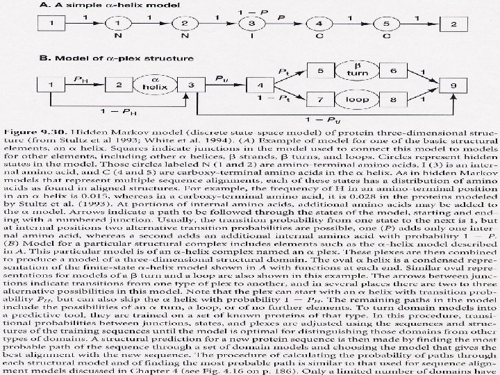
Hidden Markov Models for 2 D and 3 D Hidden Markov Models (HMMs) are a more sophisticated form of profile analysis. Rather than build a table of amino acid frequencies at each position, they model the transition from one amino acid to the next.

Homology Modeling If two proteins show sufficient sequence similarity, it essentially guarantees that they adopt the same structure. Safe thresholds: >50% identity over 25 residues >30% identity over 50 residues >25% identity over 80 residues or more If one of the two similar proteins has a known structure, can build a rough model of the protein of unknown structure. Quality of the model diminishes with lower sequence identity.

Steps in Homology Modeling 1. Do sequence alignment with protein of known structure Known Structure: ksedemkase- - dlkkhgatvltalg ||||: |: || Unknown Structure: ||: ||||||| kseddmrrseafgctytcdlrkhgntvltalg 3. Rebuild loops where there are gaps in the aligment 2. Replace any side chains that are different in the homolog (green side chains) 4. Adjust side-chains to accommodate the new residues and loops 5. Energy Minimize

3*6 environments Data from known library (AA Residues) Structure 3 D Profile Method (or 3 D-1 D method)

Threading Protein Structures Best bet is to compare with similar sequences that have known structures >> Threading u Only works for proteins with >25% sequence similarity to a protein with known structure u Current state of the art requires many days of computing on a dedicated workstation u Some websites offer quick approximations u Will improve as more 3 -D structures are described Another aspect of the Genome Project

Monte Carlo Algorithm for 3 D X: set of atomic coordinates or mainchain-sidechain torsion angles of a protein. E(x): conformation energy; k is Boltzmann’s constant; T is an effective temperature Metropolis Algorithm 1. generate a random state x, calculate E(x) 2. perturb x: x x’, to generate a neighbouring conformation 3. calculate E(x’) 4. If E(x) > E(x’), accept x’ as a new state. (downhill). Otherwise accept x’ with a probability exp(-(E(x’)-E(x))/k. T). (uphill) 5. return to 2