Protein NMR IV Isotopic labeling The only nuclei

Protein NMR IV - Isotopic labeling • The only nuclei that we can look in a protein is usually the 1 H. In small proteins (up to 10 KDa, ~ 80 amino acids) this is OK. We can identify all residues and study all NOEs, and measure most of the 3 J couplings. • As we go to larger proteins (> 10 KDa), things start getting more and more crowded. We start loosing too many residues to overlap, and we cannot assign the whole backbone chain. • What we need is more NMR sensitive nuclei in the sample. That way, we can edit the spectra by looking at those, or, for example, add a third (and maybe fourth) dimension. • To do this we need several things: a) We need to know the gene (DNA chunk) that is responsible for the synthesis of our proteins. b) We need a molecular biologist to get a plasmid that overexpresses this gene, possibly in an E. coli vector system in minimal media, so that even Joe Blow, the new (and clueless) undergrad in the lab, can grow lots of it. c) The overexpressed protein has to be functional (85% of the time you get a beautiful band in the SDS-gel that is all inclusion bodies…). d) A good/simple purification procedure.

Isotopic labeling (continued) • 10 to 1 that your particular protein will fail one of these requirements in real life. But most of the time, we can work around either overexpression, activity and purification problems. Getting the gene is the toughest one to overcome. • In any case, now that we have the plasmid, we grow it in isotopically enriched media. This usually means M 9 (minimal media), which only has NH 4 Ac and glucose as sources of N and C. No cell homogenates or yeast extracts. • So, if we want a 15 N labeled protein, we use 15 NH 4 Ac (that is dirt-cheap). Glucose-U-13 C is a lot more expensive, but it is sometimes necessary. • In that way we get partially- or fully-labeled protein, in which all nuclei are NMR-sensitive (13 C=O, 13 Ca, and 15 Ns). All the protein backbone is NMR-sensitive. H 15 N AA 2 O 13 13 C AA 1 C 13 15 N H C H 15 13 C O N O 13 13 C C AA 3 • Another cool thing is that we now have new 3 J-couplings to use for dihedral angles: H-C-C-15 N, H-N-C-13 C. These have their own Karplus parameters.

Isotopic labeling (…) • One of the most common experiments performed in 15 Nlabeled proteins is a 15 N-1 H hetero-correlation. Instead of doing the normal HETCOR which detects 15 N (low sensitivity), we do an HSQC or HMQC, which gives us the same data but using 1 H for detection. • This experiment is great, because we can spread the signals using the chemical shift range of 15 N: 7. 0 1 H d 8. 0 “ 0”� 185. 0 15 N d 165. 0 • It is ideal for several things. One of them is measurement of amide exchange rates. • It is also good to do spin system identification: If we don’t have good resolution in the COSY or TOCSY and some signals are overlapped, we can use the 1 H-15 N correlation to spread the TOCSY correlations in a third dimension…

3 D NMR spectroscopy • …which brings us to 3 D spectroscopy. There is nothing to be afraid of. The principles behind 3 D NMR are the same as those behind 2 D NMR. • Basically we can think of them this way: In the same fashion that an evolution time t 1 gave us the second dimension f 1, we can add another evolution time (which will be in the end t 1), and obtain a third frequency axis after some sort of math transformation. • For a 2 D we had: Preparation Evolution Acquisition Mixing t 1 t 2 f 1 f 2 • For a 3 D we will have: Preparation Evolution Mixing Acquisition t 1 (1) t 2 2 t 3 f 1 f 2 f 3 • As in the 2 D experiments, depending on the type of mixing we use in each chunk, the type of data we’ll get…

3 D NMR spectroscopy (continued) • We will not try to go pulse by pulse seeing how they work, but just mention (and write down) some of the sequences, and understand how they are analyzed. • We first have to separate into different categories depending on the type of mixing:

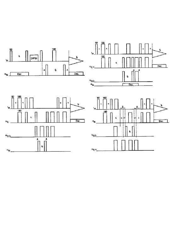
TOCSY-HSQC combination • The experiment that we used in this explanation is one of the most employed ones when doing 3 D spectroscopy, a combo of TOCSY and HSQC. The pulse sequence looks like this: 90 13 C 15 N D {1 H} 90 t 2 D {1 H} : 90 90 t 1 90 180 DIPSI 1 H: t 3 • Briefly, the first chunk is a TOCSY in 1 H, in which we have to decouple either 13 C or 15 N (yes, that means saturating these nuclei). Here we have t 1 (f 1), meaning that we’ll have a 1 HTOCSY like spectrum in this dimension. • The second part is an inversely detected HETCOR, in which we will have 1 H frequencies in one axis (f 1), and 13 C or 15 N frequencies in f 2. • Finally, detection in t 3 is in 1 H, so we have 1 H shifts and couplings in f 3.

TOCSY-HSQC combination • In a similar way we can combine a NOESY with the HSQC. The sequence is this one below: 90 13 C 15 N D {1 H} 90 t 2 D {1 H} : 90 90 t 1 90 180 tm 1 H: t 3 • Now instead of a TOCSY on the first part we have a NOESYtype deal. The second part is identical to the other one. • In the 3 D we will have a normal 1 H-15 N (or 13 C) correlation in the f 1 -f 2 plane, and NOESY planes for the f 1 -f 3 planes. It of these NOESY planes will have only a few protons. If the resolution is good, each proton has its own f 1 -f 3 plane • In the same way we can combine any other type of 2 D experiment to obtain a 3 D experiment. These two are the most used ones in proteins, which are the molecules for which 3 Ds are used the most…

Selective pulses • Many other 3 D sequences are used to identify spin systems at the beginning of the assignment process. Most of these rely in some sort of selective excitation of part of the spin systems present in the peptide. • For example, we may want to see what is linked to the Ha but not to the NHs. Also, upon labeling the peptide completely we may want to select how the transfer of magnetization goes through the peptide backbone. • In order to do such a thing we need selective pulses, which we have mentioned before, but never described in detail. • A non-selective pulse is very short and square, which in turn makes it affect frequencies to the side of the carrier due to the frequency components it has (we saw all this…). On the other hand, a selective pulse is a lot longer in time, which makes the range of frequencies a lot narrower:

Selective pulses • A problem of using longer square pulses as selective pulses is that we still have the wobbles to the sides (remember the FT of a square pulse). Therefore we are still tickling more frequencies than what we would like. • What we have to do figure a pulse in the time domain that will almost exclusively affect only certain frequencies. This means that our pulse will have a certain intensity profile versus time different from a square, and is therefore shaped. • The easiest way to obtain a shaped pulse is to see how it should look in the frequency domain (what frequencies we need it to affect), and then do a inverse Fourier Transform to the time domain: • We usually get Gaussian and squared Gaussian shaped pulses. By changing both the shape, power, and length we can tune them to affect, for example, only the Ha, the NH, the 13 C=O, or the 13 Ca regions of the spectrum…

3 D experiments using selective pulses • …which brings us back to the use of selective pulses in 3 D spectroscopy.