Propositional Logic and Resolution Dave Touretzky Read Sections

Propositional Logic and Resolution Dave Touretzky Read Sections 7. 1 - 7. 5 of Russell & Norvig

The Big Picture General Search: states are arbitrary CSPs structured states: vars ∊ domains constraint propagation Constraint Manipulation: cycle cutset; tree decomposition Satisfiability: variables ∊ {true, false} constraints = logical formulae Constraint Manipulation: resolution theorem proving 2

Logical Reasoning as CSP Find variable assignments (“models”) that satisfy all constraints. Wumpus World Bij = breeze felt Sij = stench smelt Pij = pit here Wij = wumpus here G = gold 3

Constraint Language: Syntax ● Sentence: atomic or complex ● Atomic sentence: P, Q, R, …, True, False ● Complex sentence: ○ ○ ○ (Sentence) | [Sentence] ¬ Sentence ∧ Sentence ∨ Sentence ⇒ Sentence ⇔ Sentence “negation” “conjunction” “disjunction” “implies” / “if-then” “biconditional” / “iff” 4

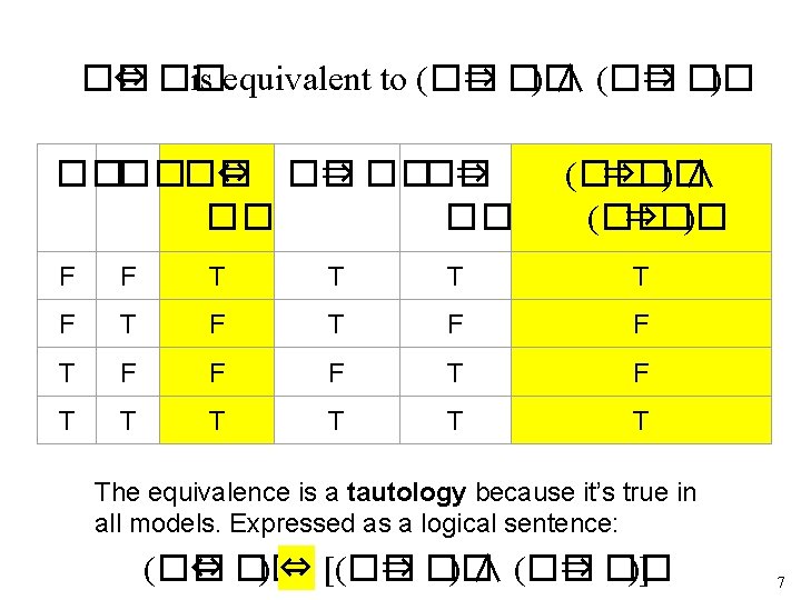
Notes on Connectives �� ∨ �� is inclusive or, not exclusive �� ⇒ �� is equivalent to ¬�� ∨ �� – Says who? �� ⇔ �� is equivalent to (�� ⇒ �� ) ∧ (�� ⇒ �� ) – Prove it! 5

�� ⇒ �� is equivalent to ¬�� ∨ �� �� ⇒ �� ¬�� ∨ �� F F T T T T T F F T T T F T When two expressions produce the same result in all possible models, their equivalence is a tautology. 6

Literals • Positive literal: P • Negative literal: ¬ P • Literals represent simple claims about the world. • Literal sentences are unary constraints on the model. Literal (Unary Constraint) Model P P = True ¬P P = False 8

Sentences As Constraints A sentence with n variables functions as an nary constraint on possible models: [(p ∧ ¬q) ∨ (q ∧ ¬p)] ⇒ r Possible Models P Q R false false true false true true true 9

Semantics: Entailment • �� ⊨ �� if and only if, in every model in which �� is true, �� is also true. • M(�� ) denotes the set of all models of ��. • �� ⊨ �� means M(�� ) ⊆ M(�� ) 10

Semantics: Grounding 11

Inference By Model Checking �� 1 is models with no pit at 1, 2. �� 1 = M(¬P 1, 2) At 1, 1: nothing. ¬P 1, 1 , ¬B 1, 1 At 2, 1: breeze B 2, 1 , ¬P 2, 1 KB Constraints: P 2, 1⇒ B 1, 1∧B 2, 2∧ B 3, 1 B 2, 1⇔ P 1, 1∨ P 2, 2 ∨P 3, 1 All models consistent with KB and constraints. M(KB) ⊆ M(�� 1. Conclude ¬ P 1, 2. 1) so KB ⊧ �� 12

Inference By Model Checking �� 2 is models with no pit at 2, 2 �� 2 = M(¬P 2, 2) At 1, 1: nothing. ¬P 1, 1 , ¬B 1, 1 At 2, 1: breeze B 2, 1 , ¬P 2, 1 KB Constraints: P 2, 1⇒ B 1, 1∧B 2, 2∧ B 3, 1 B 2, 1⇔ P 1, 1∨ P 2, 2 ∨P 3, 1 All models consistent with KB and constraints. M(KB) ⊈ M(�� 2. Can’t conclude ¬ P 2, 2. 2) so KB ⊭ �� 13

Wumpus World Agent Step 1 Agent Action Start at 1, 1. Sense: nothing. Model check. Relevant constraints: P 2, 1 ⇒ B 11 , P 1, 2 ⇒ B 11 Constraint is false in any model with P 2, 1. So KB ⊧ ¬ P 2, 1. Similarly, KB ⊧ ¬ P 1, 2. 2 Agent moves to 2, 1. Sense: breeze. Model check. Relevant constraints: B 2, 1 ⊧ P 1, 1 ∨ P 2, 2 ∨ P 3, 1 There could be a pit at 2, 2 or 3, 1 or both. Can’t infer any new literals. Tell KB (variable assignment) ¬ P 1, 1 , ¬ B 1, 1 ¬ P 2, 1 , ¬ P 1, 2 B 2, 1 -- 14

Wumpus World Agent Step Agent Action 3 Agent returns to 1, 1. 4 Agent moves to 1, 2. Sense stench, no breeze. Model check. Relevant constraints: P 2, 2 ⇒ B 12 , P 1, 3 ⇒ B 12 Constraint is false in any model with P 2, 2. So KB ⊧ ¬ P 2, 2. Similarly, KB ⊧ ¬ P 1, 3. Another relevant constraint: B 1, 2 ⇔ (P 1, 1 ∨ P 2, 2 ∨ P 3, 1) Constraint propagation gives: P 3, 1. Tell KB (variable assignment) -¬ B 1, 2 ¬ P 2, 2 , ¬ P 1, 3 P 3, 1 15

Cost of Model Checking Inference • A 4 x 4 wumpus world has 16 squares. • Four variables per square: Pij, Bij, Sij, Wij – There are 64 variables. • Search space is 264 possible models! – This could take a while… • What can we do? 16

Option 1: Exploit Locality • A constraint only references a square and its four neighbors. – Solve subproblems for smaller regions. – Share variable assignments across subproblems to get a global solution. • Constraints on P/B don’t mention S or W. Constraints on S/W don’t mention P or B. – Separate the P/B and S/W models. – Reduces state space from 2 n to 2× 2 n/2. 17

Option 2: Go Meta • Instead of searching the space of models, let’s search the space of constraints (logical formulae). • Adopt inference rules to derive new formulae from old. – This is called theorem proving. • Deriving new literals will directly give us valid models. 18

Inference Rule 1: Modus Ponens Latin for “mode that affirms”. �� ⇒ �� , �� __________ �� 19

Inference Rule 2: And-Elimination �� ∧ �� ________ �� 20

Inference Rule 3: And-Introduction �� , �� ________ �� ∧ �� 21

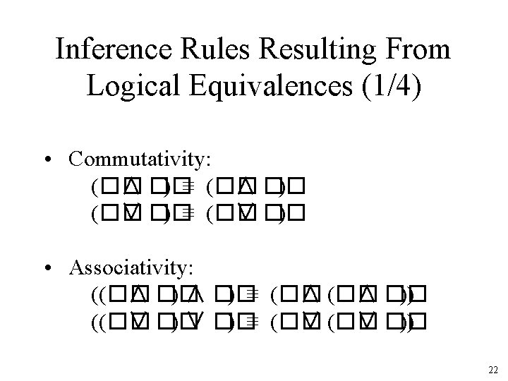
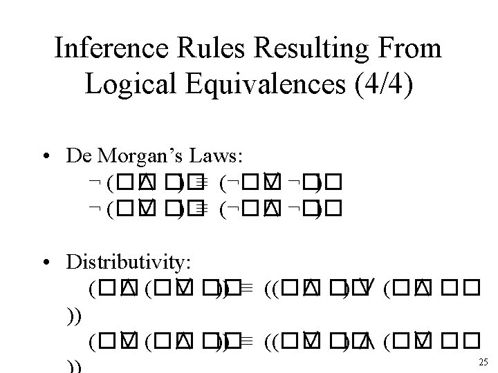
Inference Rules Resulting From Logical Equivalences (2/4) • Double-negation elimination: ¬(¬�� ) ≡ �� • Contraposition: (�� ⇒ �� ) ≡ (¬�� ⇒ ¬�� ) 23

Inference Rules Resulting From Logical Equivalences (3/4) • Implication elimination: (�� ⇒ �� ) ≡ (¬�� ∨ �� ) • Biconditional elimination: (�� ⇔ �� ) ≡ ((�� ⇒ �� ) ∧ (�� ⇒ �� )) 24

Proof: From ¬B 1, 1 Derive ¬P 2, 1 1 ¬ B 1, 1 Given 2 B 1, 1 ⇔ (P 1, 2 ∨ P 2, 1) Wumpus constraint (given) 3 (B 1, 1 ⇒ (P 1, 2 ∨ P 2, 1)) ∧ ((P 1, 2 ∨ P 2, 1) ⇒ B 1, 1) Biconditional elimination from 2 4 (P 1, 2 ∨ P 2, 1) ⇒ B 1, 1 And-Elimination from 3 5 ¬B 1, 1 ⇒ ¬(P 1, 2 ∨ P 2, 1) Contrapositive from 4 6 ¬ (P 1, 2 ∨ P 2, 1) Modus ponens from 1 + 5 7 (¬P 1, 2 ∧ ¬P 2, 1) De Morgan from 6 8 ¬P 2, 1 And-Elimination from 7 26

Soundness and Completeness • Entailment: �� ⊧ �� means �� is true in all models of ��. • Derivation: �� ⊦I �� means �� can be derived from �� using the inference rules in I. • Soundness of I: if �� ⊦I �� then �� ⊧ �� – Using I, we only derive entailed sentences. – “We don’t make stuff up. ” • Completeness of I: if �� ⊧ �� then �� ⊦I �� – All entailed sentences are derivable using I. – “If it’s true, we can deduce it. ” 27

Validity and Satisfiability • A sentence �� is valid if it is true in all models. We denote this by ⊧��. • A sentence �� is satisfiable if it is true in at least one model. • If a sentence �� is valid, its negation ¬�� is not satisfiable. – To prove �� , show that ¬�� is unsatisfiable. 28

Theorem Proving • Start with axioms and givens, and apply inference rules to derive new formulae. • But there are O(2 N) formulae in N vars! • And most are useless. • How can we focus on formulae relevant to proving our goal? 29

Resolution Theorem Proving • The good news: there is a single inference rule that is sound, complete, and can find proofs with reasonable efficiency. • The bad news: it only works for problems in conjunctive normal form. • But any sentence can be rewritten in conjunctive normal form. • … but length may increase exponentially. 30

Definition: Clause A clause is a disjunction of literals: l 1 ∨ l 2 ∨ … ∨ ln The li may be positive or negative. A single literal l is called a unit clause. 31

Definition: Conjunctive Normal Form A sentence is in conjunctive normal form if it is a conjunction of clauses: c 1 ∧ c 2 ∧ … ∧ cm Example: (P ∨ ¬Q ∨ R) ∧ (Q ∨ S) ∧ (P ∨ ¬R ∨ T) 32

Converting to CNF B 1, 1 ⇔ (P 1, 2 ∨ P 2, 1) Given (B 1, 1 ⇒ (P 1, 2 ∨ P 2, 1)) ∧ ((P 1, 2 ∨ P 2, 1) ⇒ B 1, 1) Biconditional elimination (¬B 1, 1 ∨ P 1, 2 ∨ P 2, 1) ∧ (¬(P 1, 2 ∨ P 2, 1) ∨ B 1, 1) Implication elimination (twice) (¬B 1, 1 ∨ P 1, 2 ∨ P 2, 1) ∧ ((¬P 1, 2 ∧ ¬P 2, 1) ∨ B 1, 1) [ (¬B 1, 1 ∨ P 1, 2 ∨ P 2, 1) ∧ (¬P 1, 2 ∨ B 1, 1 ) ∧ (¬P 2, 1 ∨ B 1, 1) ] De Morgan Distributivity Result is in CNF. 33

Converting to CNF (a ∧ b) ∨ (c ∧ d) ∨ (e ∧ f) This sentence happens to be in DNF. converts to (a ∨ c ∨ e) ∧ (a ∨ c ∨ f) ∧ (a ∨ d ∨ e) ∧ (a ∨ d ∨ f) ∧ (b ∨ c ∨ e) ∧ (b ∨ c ∨ f) ∧ (b ∨ d ∨ e) ∧ (b ∨ d ∨ f) ∧ 34

The Resolution Inference Rule l 1 ∨ l 2 ∨ … ∨ lk , m 1 ∨ m 2 ∨ … ∨ mn ____________________________ l 1 ∨ … ∨ li-1 ∨ li+1 ∨ … ∨ lk ∨ m 1 ∨ … ∨ mj-1 ∨ mj+1 ∨ … ∨ mn where li and mj are complementary literals, i. e. , li is ¬mj. From two clauses of length k and n, derives a new clause of length k+n-2. 35

Resolution Example P 1, 1 ∨ P 2, 2 ∨ P 3, 1 , ¬P 2, 2 ____________________ P 1, 1 ∨ P 3, 1 36

Contradictions Generate An Empty Clause • P ∧ ¬P is a contradiction, and therefore unsatisfiable. • Resolving P with ¬P yields an empty clause. P , ¬P ___________ � 37

Wumpus Reasoning by Resolution Not a horn clause Tautology (useless) To prove ¬P 1, 2, add P 1, 2 to the set of givens and use resolution to derive a contradiction. 38

More Efficient Inference • Resolution is complete, but even with only one inference rule, the worst case cost is exponential in the # of symbols. • But for problems that can be formulated using Horn clauses, inference can be more efficient. • With definite clauses entailment can be decided in linear time. 39

Horn Clauses • A Horn clause is a clause with at most one positive literal. • A definite clause has exactly one. – Example: (¬q 1 ∨ ¬q 2 ∨ … ∨ ¬qn ∨ p) • The positive literal p is called the head. • A definite clause is equivalent to: (q 1 ∧ q 2 ∧ … ∧ qn) ⇒ p 40

Reasoning With Horn Clauses • Clauses consisting of a single positive literal are called facts. • A clause with no positive literals is called a goal. • Horn clauses are closed under resolution. 41

Forward Chaining Algorithm • Requires the KB to consist of definite clauses (exactly one positive literal): – Facts: q 1, q 2, … – Rules: (¬q 1 ∨ ¬q 2 ∨ … ∨ ¬qn ∨ p) • Produces only positive conclusions. • Generates conclusions until goal is reached. • Runs in linear time. 42

Backward Chaining Algorithm • KB must contain only definite clauses. – Start with a goal query q. – Find the rules whose conclusion is q. – Try to recursively prove the antecedents of each rule. • Only looks at facts relevant to the query q. • Runs in linear time; is often very fast. 43

Summary • Propositional logic is a constraint language. • Model checking can be tractable if you can exploit locality in the state space. • Propositional entailment is co-NP Complete, so worst case is O(2 N). • In practice, many problems can be solved efficiently by resolution, especially if they can be formulated using definite clauses. 44