Properties of Demand Functions u Comparative statics analysis

Properties of Demand Functions u Comparative statics analysis of ordinary demand functions: The study of how ordinary demands x 1*(p 1, p 2, y) and x 2*(p 1, p 2, y) change as prices p 1, p 2 and income y change.

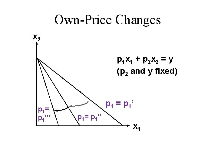
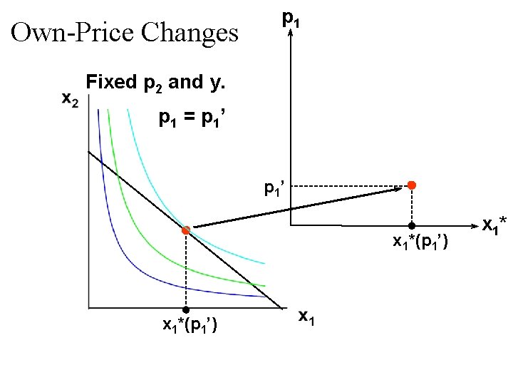
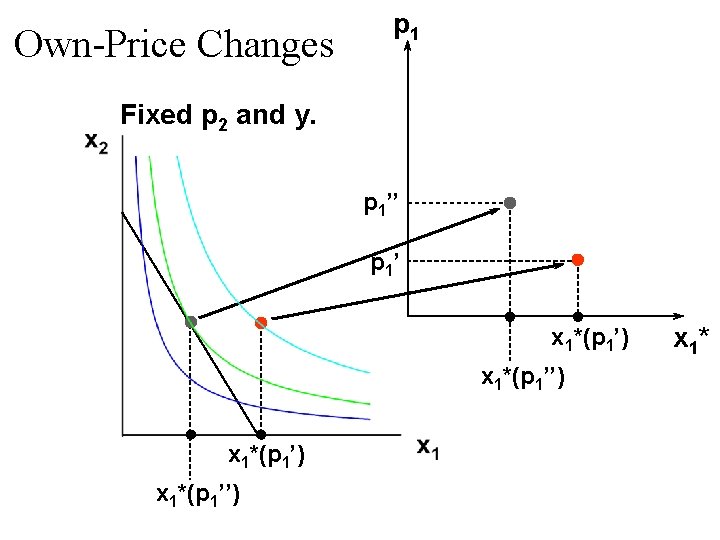
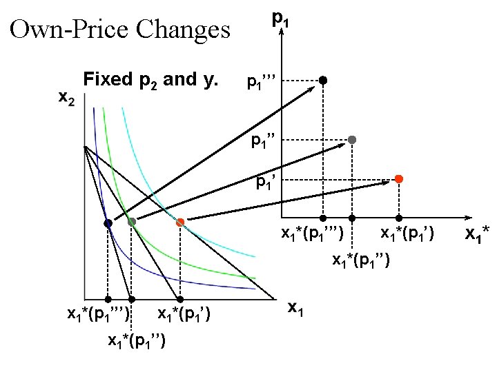
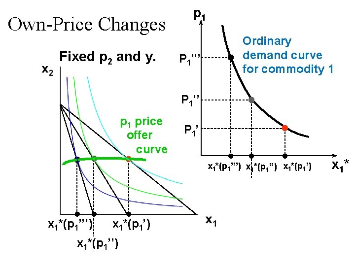
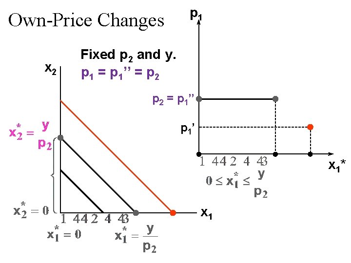
Own-Price Changes u How does x 1*(p 1, p 2, y) change as p 1 changes, holding p 2 and y constant? u Suppose only p 1 increases, from p 1’ to p 1’’ and then to p 1’’’.

Own-Price Changes x 2 p 1 x 1 + p 2 x 2 = y (p 2 and y fixed) p 1= p 1’’’ p 1 = p 1’ p 1= p 1’’ x 1

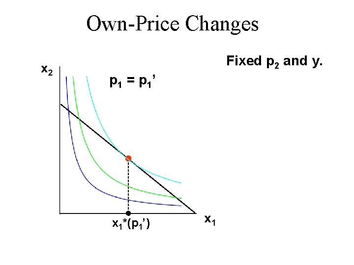
Own-Price Changes Fixed p 2 and y. p 1 = p 1’ x 1*(p 1’)

Own-Price Changes p 1 Fixed p 2 and y. p 1 = p 1’ x 1*(p 1’) x 1*

Own-Price Changes p 1 Fixed p 2 and y. p 1’’ p 1’ x 1*(p 1’) x 1*(p 1’’) x 1*

Own-Price Changes Fixed p 2 and y. p 1’’’ p 1’ x 1*(p 1’’’) x 1*(p 1’) x 1*(p 1’’) x 1*

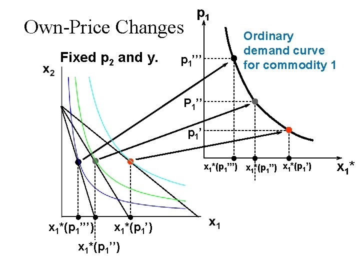
Own-Price Changes Fixed p 2 and y. p 1’’’ Ordinary demand curve for commodity 1 P 1’’ p 1’ x 1*(p 1’’’) x 1*(p 1’) x 1*(p 1’’’) x 1*(p 1’’) x 1*

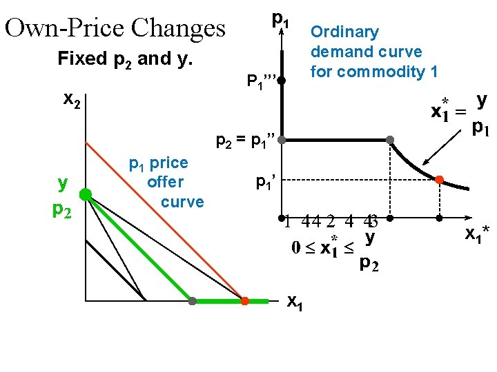
Own-Price Changes Fixed p 2 and y. p 1 P 1’’’ Ordinary demand curve for commodity 1 P 1’’ p 1 price offer curve P 1’ x 1*(p 1’’’) x 1*(p 1’) x 1*(p 1’’’) x 1*(p 1’’) x 1*

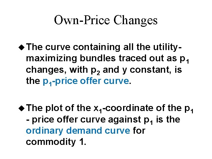
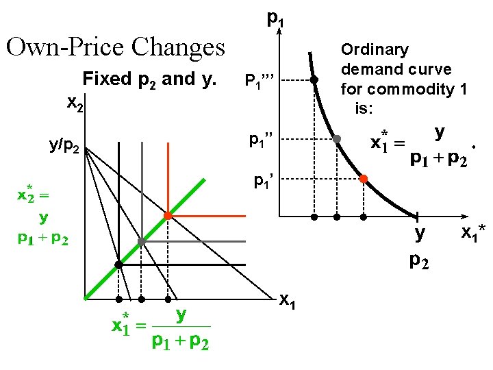
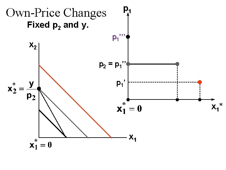
Own-Price Changes u The curve containing all the utilitymaximizing bundles traced out as p 1 changes, with p 2 and y constant, is the p 1 -price offer curve. u The plot of the x 1 -coordinate of the p 1 - price offer curve against p 1 is the ordinary demand curve for commodity 1.

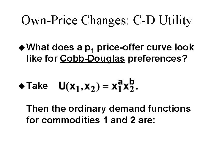
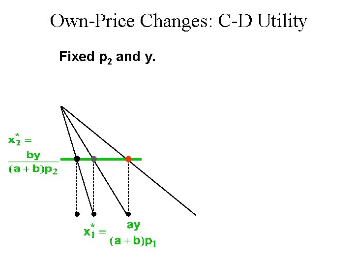
Own-Price Changes: C-D Utility u What does a p 1 price-offer curve look like for Cobb-Douglas preferences? u Take Then the ordinary demand functions for commodities 1 and 2 are:

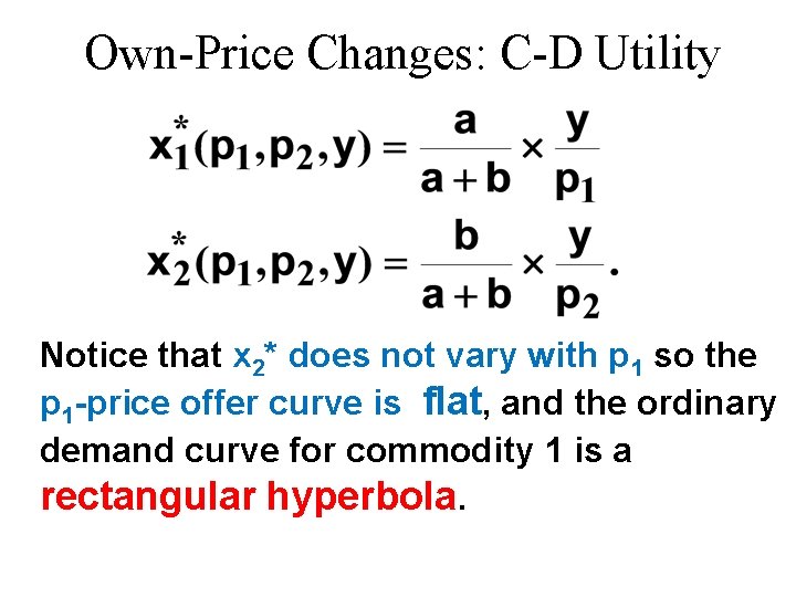
Own-Price Changes: C-D Utility Notice that x 2* does not vary with p 1 so the p 1 -price offer curve is flat, and the ordinary demand curve for commodity 1 is a rectangular hyperbola.

Own-Price Changes: C-D Utility Fixed p 2 and y. x 1*(p 1’’’) x 1*(p 1’’)

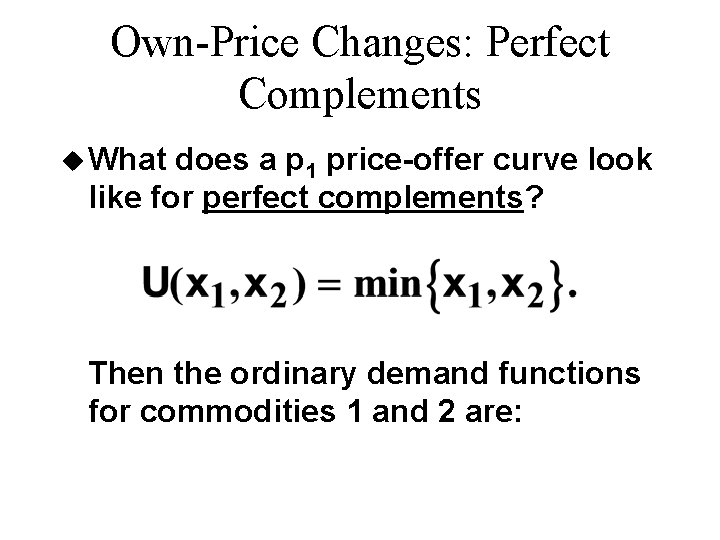
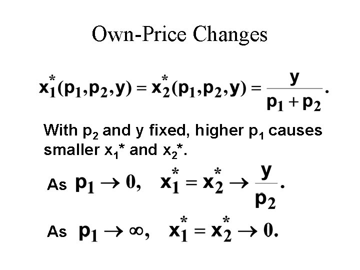
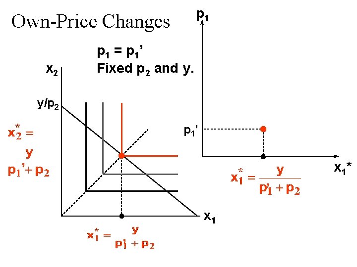
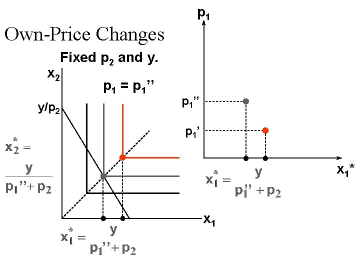
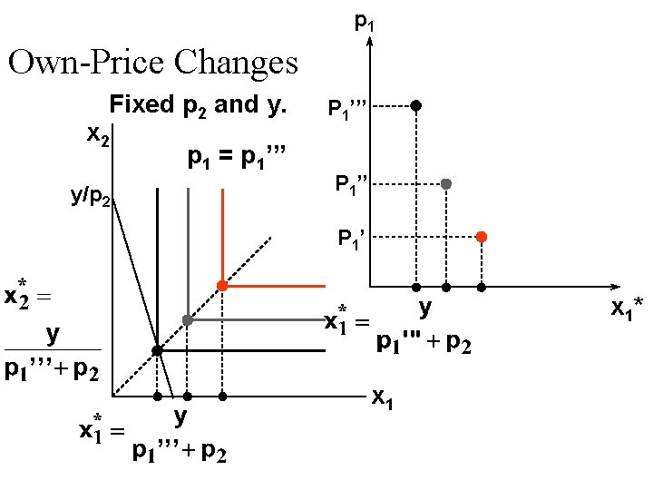
Own-Price Changes: Perfect Complements u What does a p 1 price-offer curve look like for perfect complements? Then the ordinary demand functions for commodities 1 and 2 are:

Own-Price Changes With p 2 and y fixed, higher p 1 causes smaller x 1* and x 2*. As As

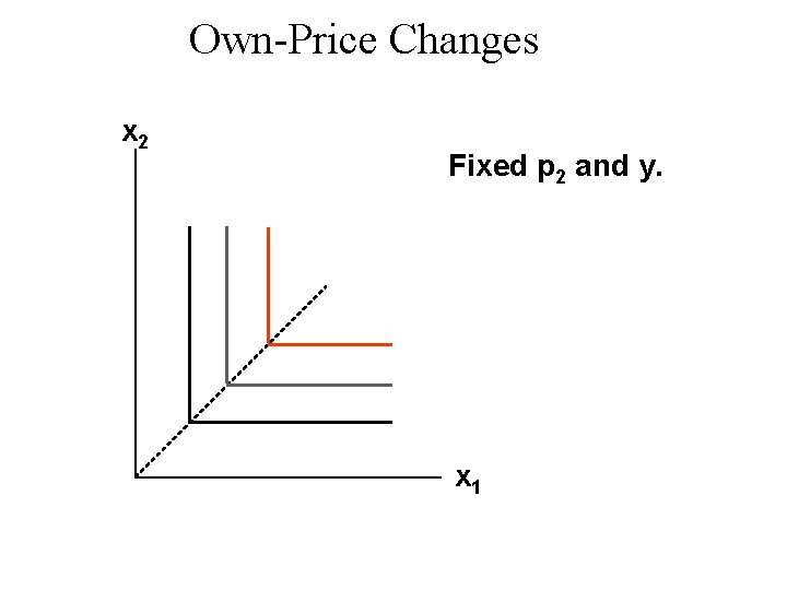
Own-Price Changes x 2 Fixed p 2 and y. x 1

p 1 Own-Price Changes x 2 p 1 = p 1’ Fixed p 2 and y. y/p 2 p 1’ x 1* ’ ’ x 1 ’

p 1 Own-Price Changes x 2 Fixed p 2 and y. p 1 = p 1’’ y/p 2 p 1’’ p 1’ x 1* ’’ ’’ x 1 ’’

p 1 Own-Price Changes Fixed p 2 and y. x 2 p 1 = p 1’’’ y/p 2 P 1’’’ P 1’ "' ’’’ x 1*

p 1 Own-Price Changes Fixed p 2 and y. x 2 y/p 2 Ordinary demand curve for commodity 1 is: P 1’’’ p 1’ x 1* x 1

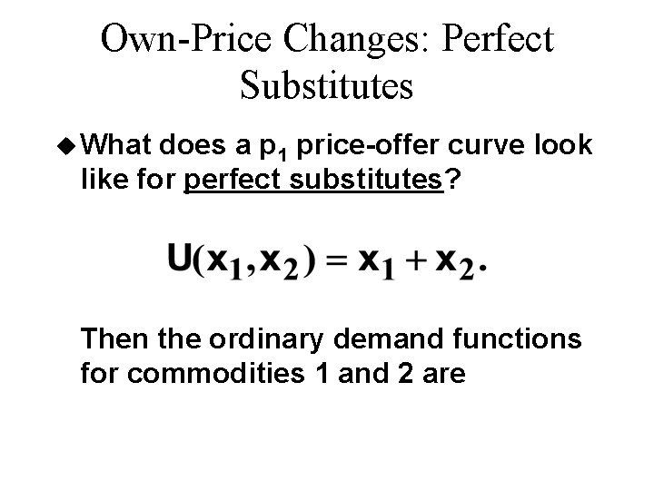
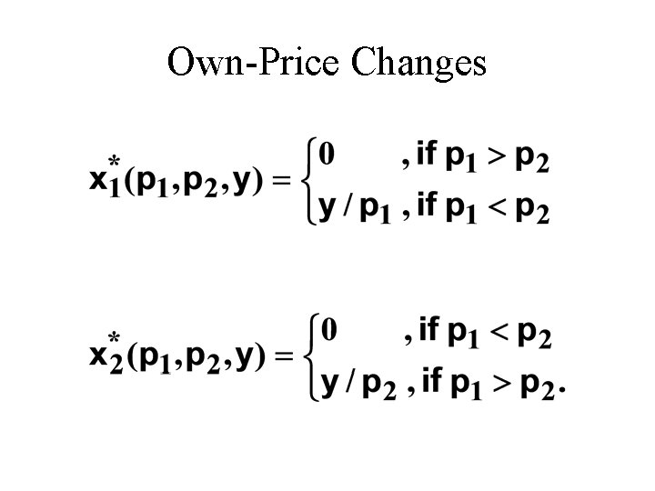
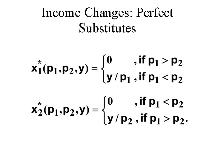
Own-Price Changes: Perfect Substitutes u What does a p 1 price-offer curve look like for perfect substitutes? Then the ordinary demand functions for commodities 1 and 2 are

Own-Price Changes

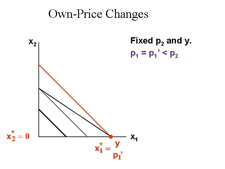
Own-Price Changes Fixed p 2 and y. p 1 = p 1’ < p 2 x 1 ’

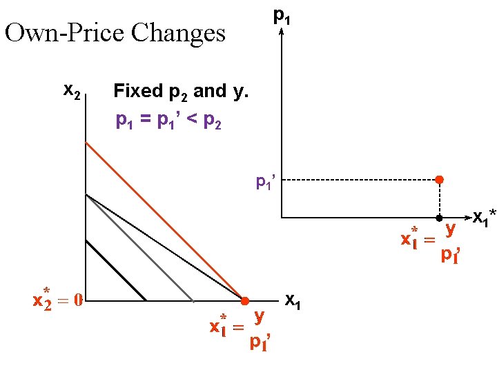
p 1 Own-Price Changes x 2 Fixed p 2 and y. p 1 = p 1’ < p 2 p 1’ x 1* ’ x 1 ’

Own-Price Changes x 2 p 1 Fixed p 2 and y. p 1 = p 1’’ = p 2 = p 1’’ p 1’ x 1* x 1

Own-Price Changes p 1 Fixed p 2 and y. x 2 p 1’’’ p 2 = p 1’’ p 1’ x 1* x 1

Own-Price Changes Fixed p 2 and y. x 2 p 1 P 1’’’ Ordinary demand curve for commodity 1 p 2 = p 1’’ p 1 price offer curve p 1’ x 1* x 1

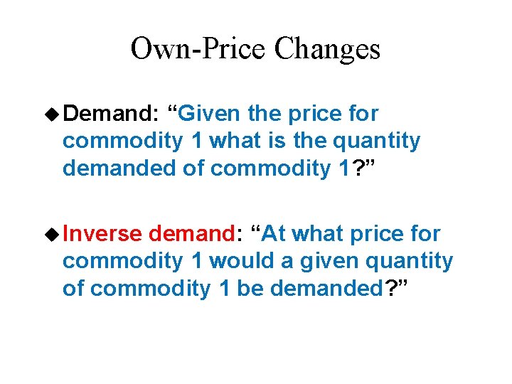
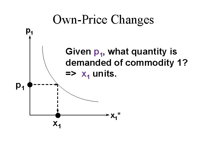
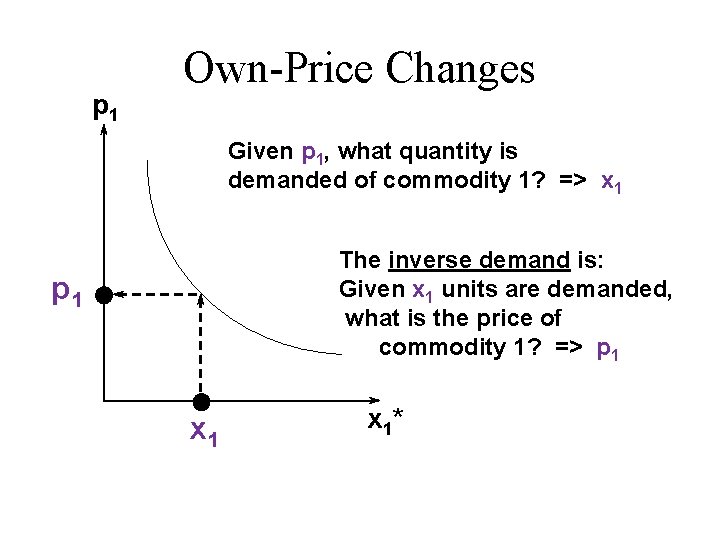
Own-Price Changes u Demand: “Given the price for commodity 1 what is the quantity demanded of commodity 1? ” u Inverse demand: “At what price for commodity 1 would a given quantity of commodity 1 be demanded? ”

p 1 Own-Price Changes Given p 1, what quantity is demanded of commodity 1? => x 1 units. p 1 x 1*

p 1 Own-Price Changes Given p 1, what quantity is demanded of commodity 1? => x 1 The inverse demand is: Given x 1 units are demanded, what is the price of commodity 1? => p 1 x 1*

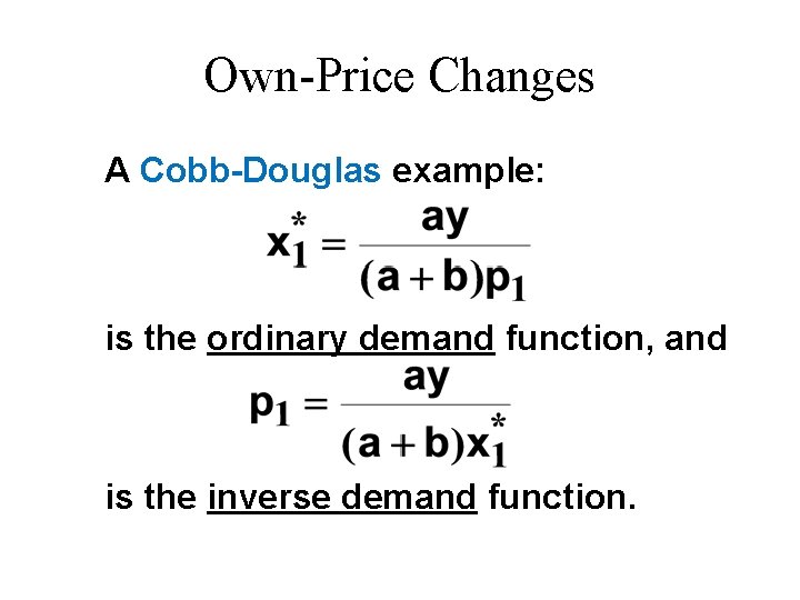
Own-Price Changes A Cobb-Douglas example: is the ordinary demand function, and is the inverse demand function.

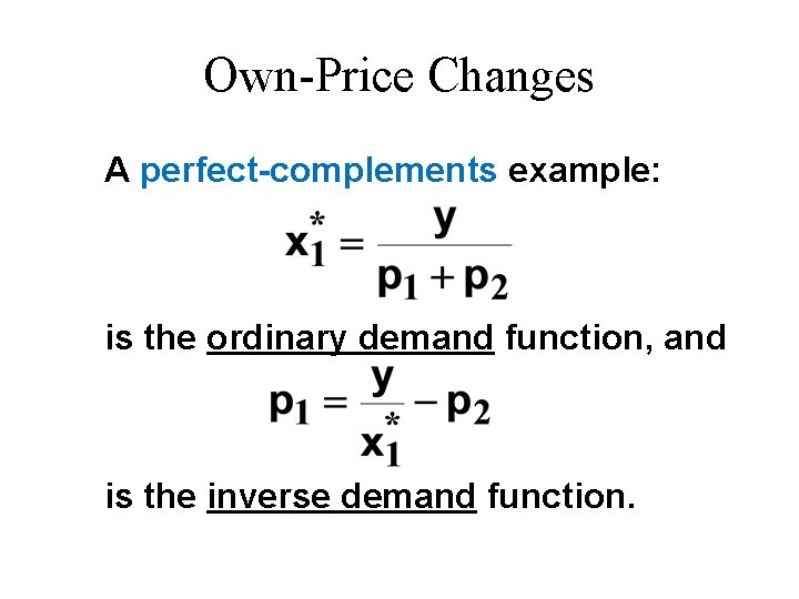
Own-Price Changes A perfect-complements example: is the ordinary demand function, and is the inverse demand function.

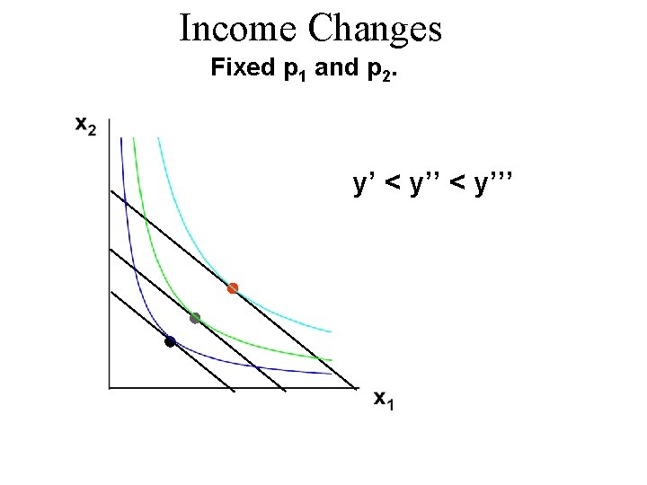
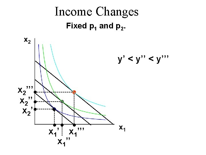
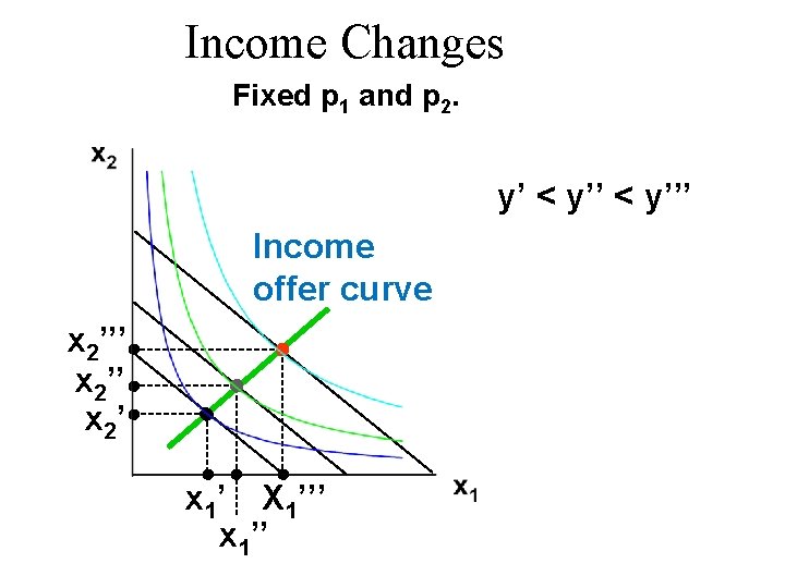
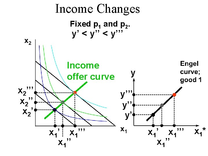
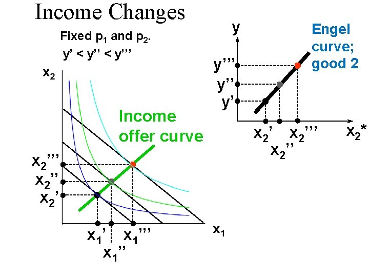
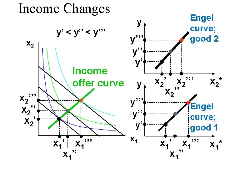
Income Changes u How does the value of x 1*(p 1, p 2, y) change as y changes, holding both p 1 and p 2 constant?

Income Changes Fixed p 1 and p 2. y’ < y’’’

Income Changes Fixed p 1 and p 2. y’ < y’’’ x 2’’ x 2’ x 1’’’ x 1’’

Income Changes Fixed p 1 and p 2. y’ < y’’’ Income offer curve x 2’’’ x 2’ x 1’ X 1’’’ x 1’’

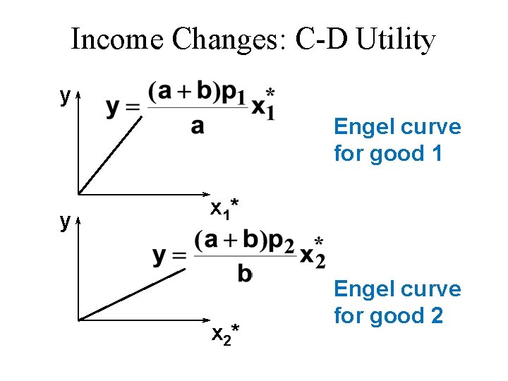
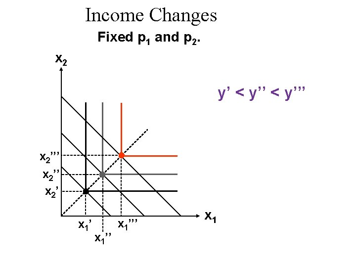
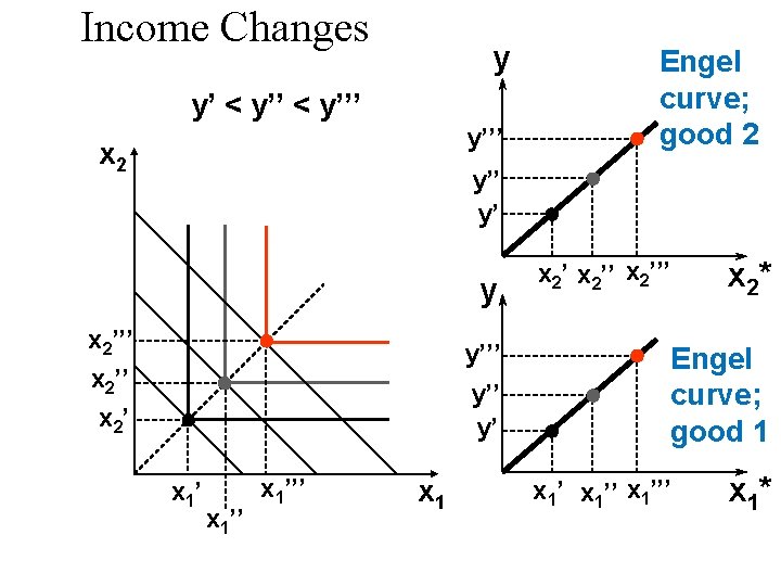
Income Changes u. A plot of quantity demanded against income is called an Engel curve.

Income Changes Fixed p 1 and p 2. y’ < y’’’ Income offer curve x 2’’’ x 2’ y y’’’ y’ x 1’’’ x 1’’ x 1*

Income Changes Fixed p 1 and p 2. y’ < y’’’ Income offer curve x 2’’’ x 2’ x 1’’’ x 1’’ y y’’’ y’ Engel curve; good 2 x 2’’’ x 2*

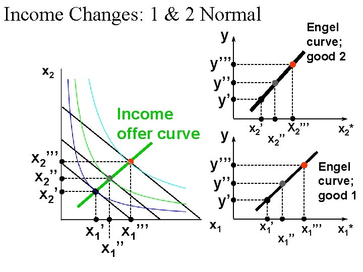
Income Changes y’ < y’’’ Income offer curve x 2’’’ x 2’ y y’’’ y’’ y’ x 1’’’ x 1’’ Engel curve; good 2 x 2’’’ x 2* Engel curve; good 1 x 1’’’ x 1* x 1’’

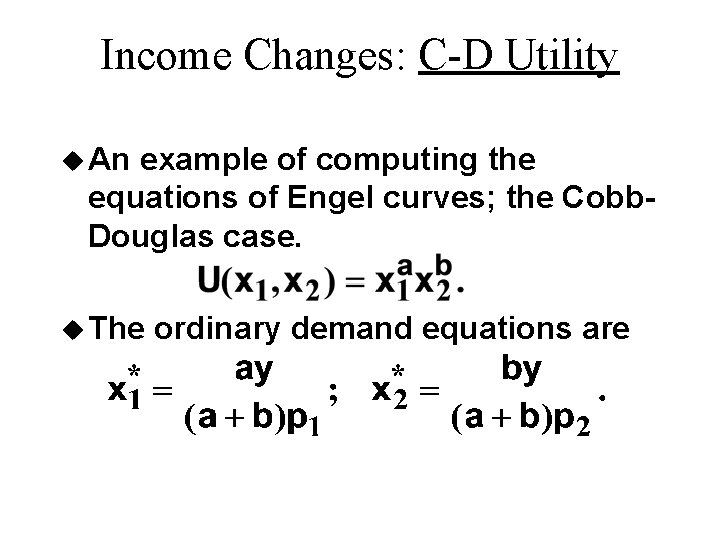
Income Changes: C-D Utility u An example of computing the equations of Engel curves; the Cobb. Douglas case. u The ordinary demand equations are

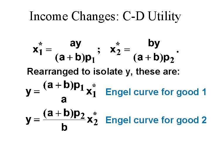
Income Changes: C-D Utility Rearranged to isolate y, these are: Engel curve for good 1 Engel curve for good 2

Income Changes: C-D Utility y Engel curve for good 1 y x 1* x 2* Engel curve for good 2

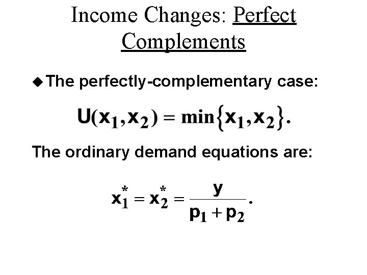
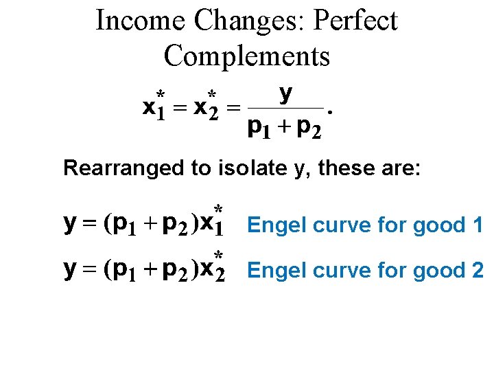
Income Changes: Perfect Complements u The perfectly-complementary case: The ordinary demand equations are:

Income Changes: Perfect Complements Rearranged to isolate y, these are: Engel curve for good 1 Engel curve for good 2

Income Changes Fixed p 1 and p 2. x 2 y’ < y’’’ x 2’’ x 2’ x 1’’’ x 1

Income Changes y y’ < y’’’ x 2 Engel curve; good 2 y’’ y’ y x 2’’’ x 2’ y’’ y’ x 1’’’ x 1 x 2’’’ x 2* Engel curve; good 1 x 1’’’ x 1*

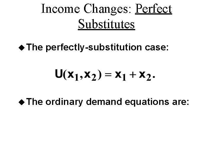
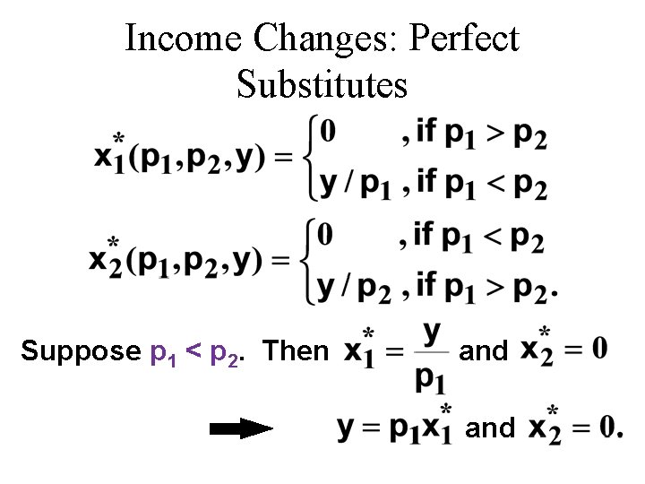
Income Changes: Perfect Substitutes u The perfectly-substitution case: u The ordinary demand equations are:

Income Changes: Perfect Substitutes

Income Changes: Perfect Substitutes Suppose p 1 < p 2. Then and

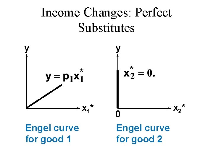
Income Changes: Perfect Substitutes y y x 1* Engel curve for good 1 0 Engel curve for good 2 x 2*

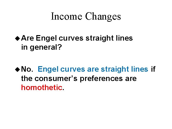
Income Changes u Are Engel curves straight lines in general? u No. Engel curves are straight lines if the consumer’s preferences are homothetic.

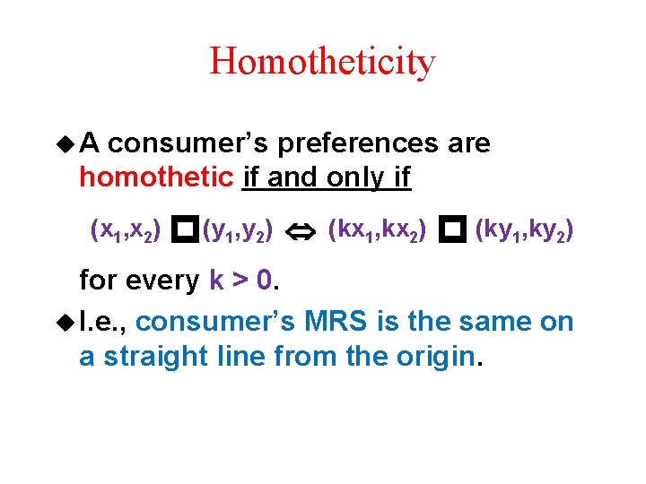
Homotheticity u. A consumer’s preferences are homothetic if and only if (x 1, x 2) p(y 1, y 2) Û (kx 1, kx 2) p (ky 1, ky 2) for every k > 0. u I. e. , consumer’s MRS is the same on a straight line from the origin.

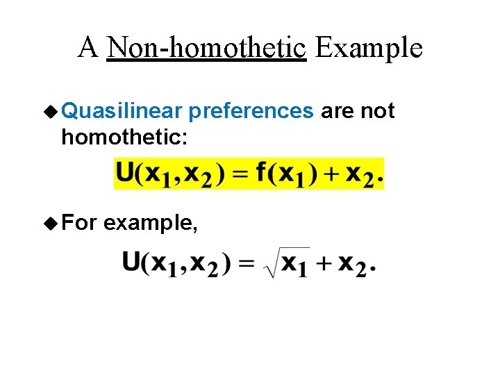
A Non-homothetic Example u Quasilinear preferences are not homothetic: u For example,

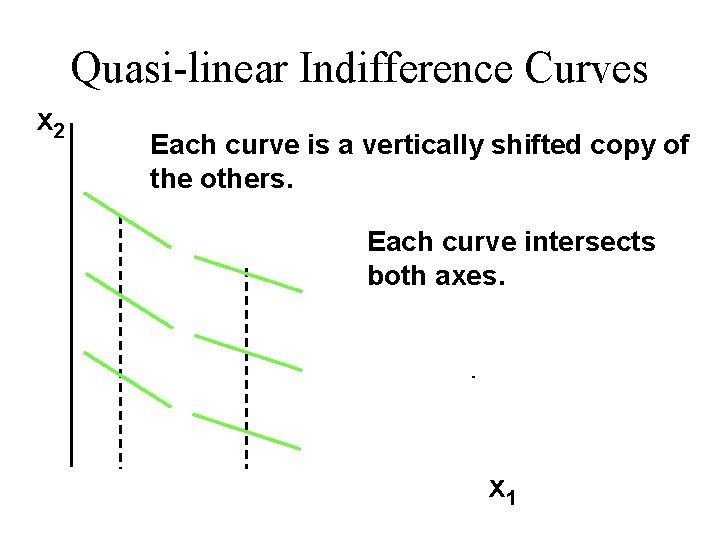
Quasi-linear Indifference Curves x 2 Each curve is a vertically shifted copy of the others. Each curve intersects both axes. x 1

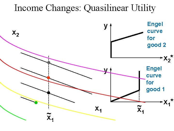
Income Changes: Quasilinear Utility Engel curve for good 2 y x 2* Engel curve for good 1 y ~ x 1 x 1*

Income Effects u. A good for which quantity demanded rises with income is called normal. u Therefore, Engel curves of normal goods are positively sloped.

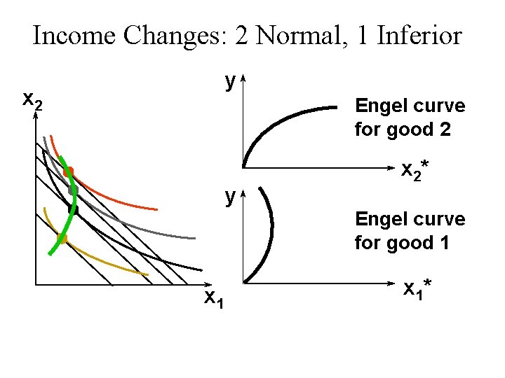
Income Effects u. A good for which quantity demanded falls as income increases is called (income) inferior. u Therefore, Engel curve of an income inferior good is negatively sloped.

Income Changes: 1 & 2 Normal Engel curve; good 2 y Income offer curve x 2’’’ x 2’ y’’ y’ y x 2’’ X 2’’’ y’’ y’ x 1’’’ x 1’’ x 2* Engel curve; good 1 x 1’’’ x 1*

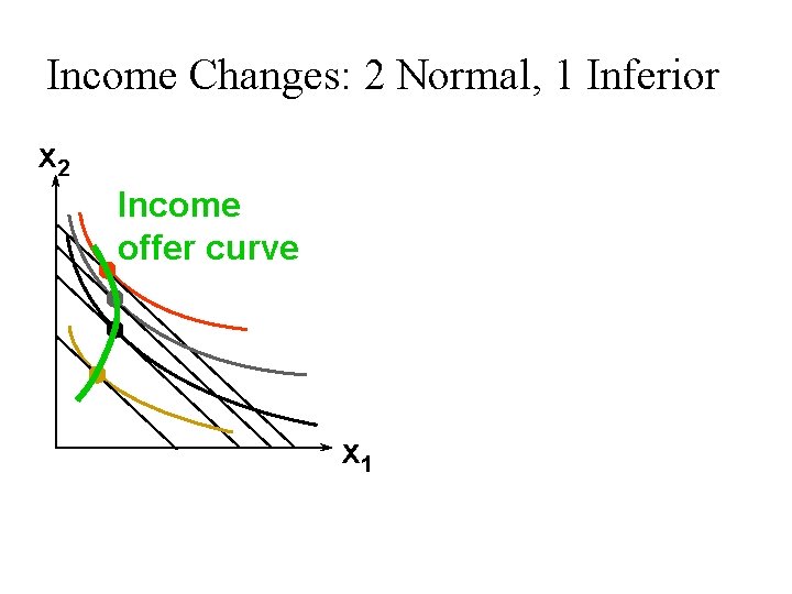
Income Changes: 2 Normal, 1 Inferior x 2 Income offer curve x 1

Income Changes: 2 Normal, 1 Inferior x 2 y Engel curve for good 2 y x 2* Engel curve for good 1 x 1*

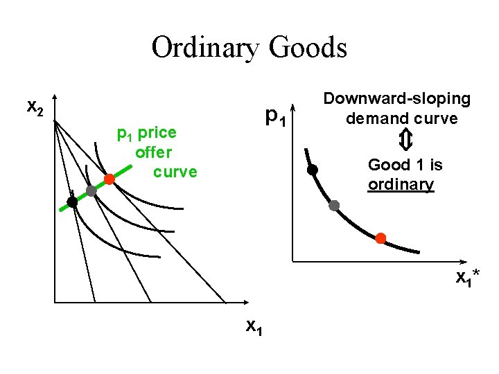
Ordinary Goods u. A good is called ordinary if the quantity demanded of it always increases as its own price decreases.

Ordinary Goods x 2 p 1 price offer curve Û p 1 Downward-sloping demand curve Good 1 is ordinary x 1* x 1

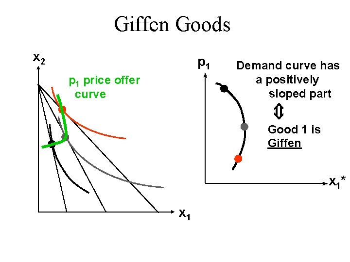
Giffen Goods u If, for some values of its own price, the quantity demanded of a good rises as its own-price increases then the good is called Giffen.

Giffen Goods x 2 p 1 price offer curve Demand curve has a positively sloped part Û Good 1 is Giffen x 1* x 1

Cross-Price Effects u If an increase in p 2 – increases demand for commodity 1, then commodity 1 is a gross substitute for commodity 2. – reduces demand for commodity 1, then commodity 1 is a gross complement for commodity 2.

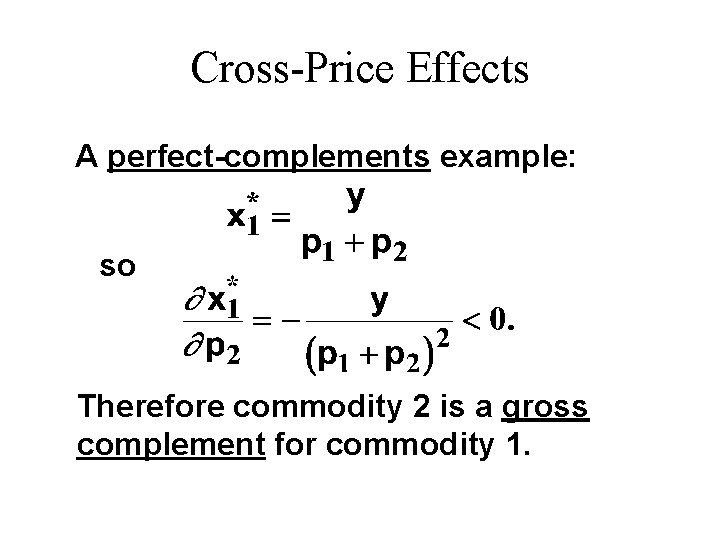
Cross-Price Effects A perfect-complements example: so Therefore commodity 2 is a gross complement for commodity 1.

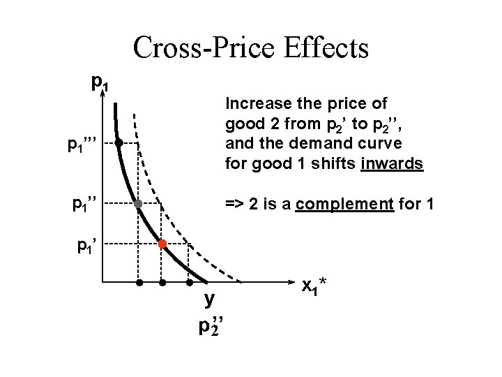
Cross-Price Effects p 1 Increase the price of good 2 from p 2’ to p 2’’, and the demand curve for good 1 shifts inwards p 1’’’ p 1’’ => 2 is a complement for 1 p 1’ x 1* ’’

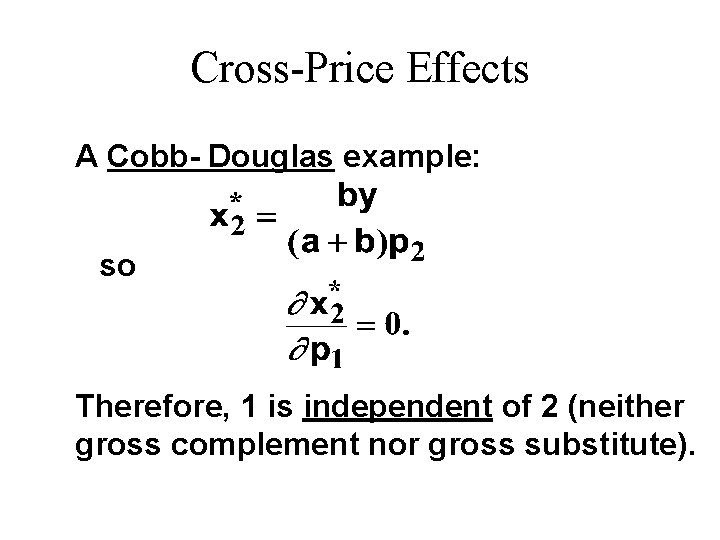
Cross-Price Effects A Cobb- Douglas example: so Therefore, 1 is independent of 2 (neither gross complement nor gross substitute).