Propagation of Error Ch En 475 Unit Operations

Propagation of Error Ch En 475 Unit Operations

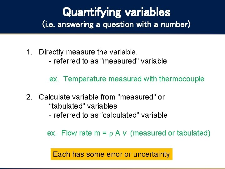
Quantifying variables (i. e. answering a question with a number) 1. Directly measure the variable. - referred to as “measured” variable ex. Temperature measured with thermocouple 2. Calculate variable from “measured” or “tabulated” variables - referred to as “calculated” variable ex. Flow rate m = A v (measured or tabulated) Each has some error or uncertainty

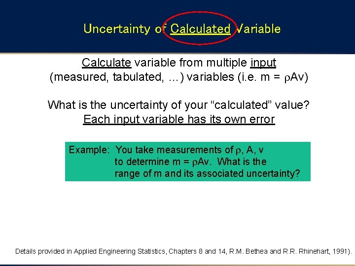
Uncertainty of Calculated Variable Calculate variable from multiple input (measured, tabulated, …) variables (i. e. m = Av) What is the uncertainty of your “calculated” value? Each input variable has its own error Example: You take measurements of , A, v to determine m = Av. What is the range of m and its associated uncertainty? Details provided in Applied Engineering Statistics, Chapters 8 and 14, R. M. Bethea and R. R. Rhinehart, 1991).

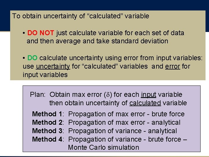
To obtain uncertainty of “calculated” variable • DO NOT just calculate variable for each set of data and then average and take standard deviation • DO calculate uncertainty using error from input variables: use uncertainty for “calculated” variables and error for input variables Plan: Obtain max error (d) for each input variable then obtain uncertainty of calculated variable Method 1: Method 2: Method 3: Method 4: Propagation of max error - brute force Propagation of max error - analytical Propagation of variance - brute force – Monte Carlo simulation

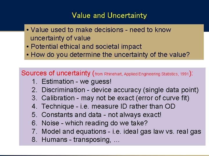
Value and Uncertainty • Value used to make decisions - need to know uncertainty of value • Potential ethical and societal impact • How do you determine the uncertainty of the value? Sources of uncertainty (from Rhinehart, Applied Engineering Statistics, 1991): 1. Estimation - we guess! 2. Discrimination - device accuracy (single data point) 3. Calibration - may not be exact (error of curve fit) 4. Technique - i. e. measure ID rather than OD 5. Constants and data - not always exact! 6. Noise - which reading do we take? 7. Model and equations - i. e. ideal gas law vs. real gas 8. Humans - transposing, …

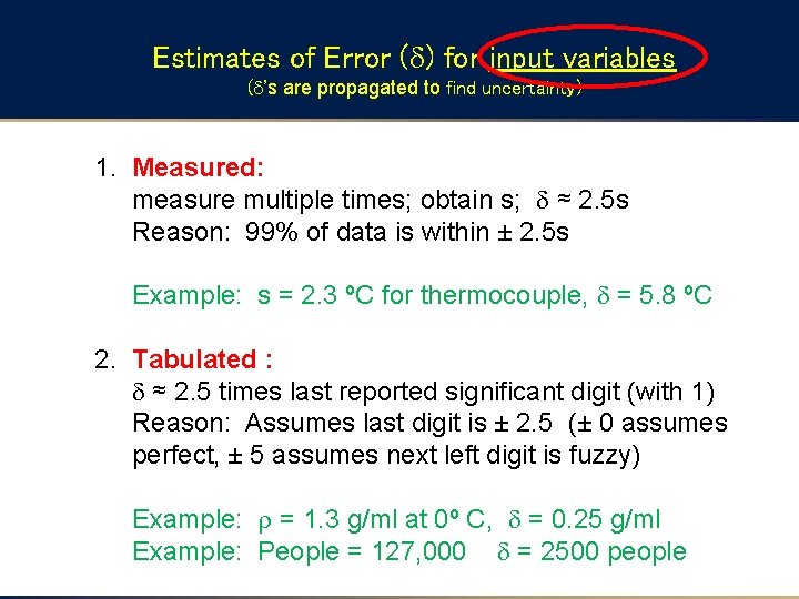
Estimates of Error (d) for input variables (d’s are propagated to find uncertainty) 1. Measured: measure multiple times; obtain s; d ≈ 2. 5 s Reason: 99% of data is within ± 2. 5 s Example: s = 2. 3 ºC for thermocouple, d = 5. 8 ºC 2. Tabulated : d ≈ 2. 5 times last reported significant digit (with 1) Reason: Assumes last digit is ± 2. 5 (± 0 assumes perfect, ± 5 assumes next left digit is fuzzy) Example: = 1. 3 g/ml at 0º C, d = 0. 25 g/ml Example: People = 127, 000 d = 2500 people

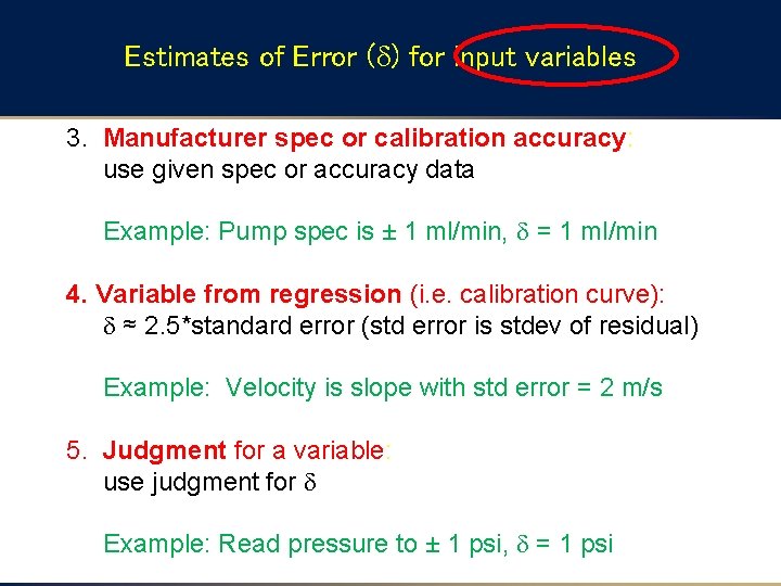
Estimates of Error (d) for input variables 3. Manufacturer spec or calibration accuracy: use given spec or accuracy data Example: Pump spec is ± 1 ml/min, d = 1 ml/min 4. Variable from regression (i. e. calibration curve): d ≈ 2. 5*standard error (std error is stdev of residual) Example: Velocity is slope with std error = 2 m/s 5. Judgment for a variable: use judgment for d Example: Read pressure to ± 1 psi, d = 1 psi

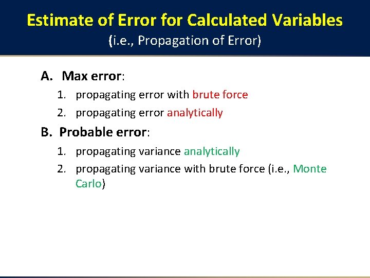
Estimate of Error for Calculated Variables (i. e. , Propagation of Error) A. Max error: 1. propagating error with brute force 2. propagating error analytically B. Probable error: 1. propagating variance analytically 2. propagating variance with brute force (i. e. , Monte Carlo)

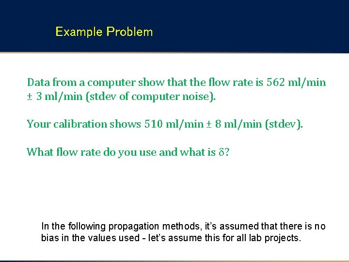
Example Problem Data from a computer show that the flow rate is 562 ml/min ± 3 ml/min (stdev of computer noise). Your calibration shows 510 ml/min ± 8 ml/min (stdev). What flow rate do you use and what is d? In the following propagation methods, it’s assumed that there is no bias in the values used - let’s assume this for all lab projects.

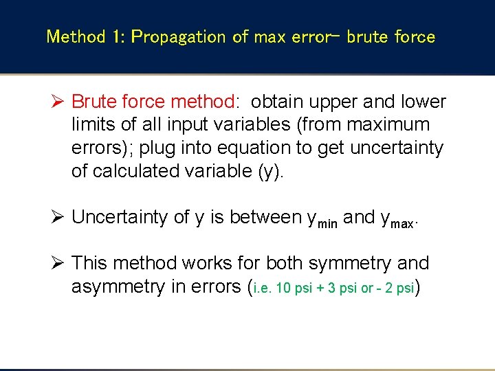
Method 1: Propagation of max error- brute force Ø Brute force method: obtain upper and lower limits of all input variables (from maximum errors); plug into equation to get uncertainty of calculated variable (y). Ø Uncertainty of y is between ymin and ymax. Ø This method works for both symmetry and asymmetry in errors (i. e. 10 psi + 3 psi or - 2 psi)

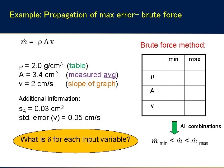
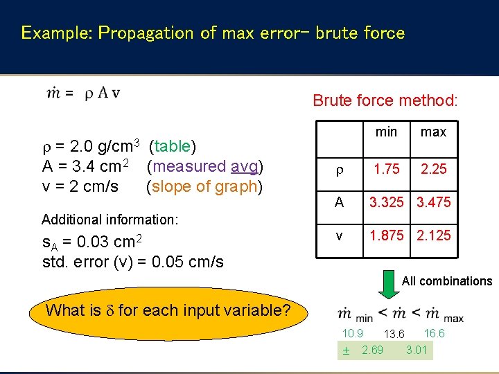
Example: Propagation of max error- brute force Brute force method: = 2. 0 A = 3. 4 cm 2 v = 2 cm/s g/cm 3 (table) (measured avg) (slope of graph) min max A Additional information: s. A = 0. 03 cm 2 std. error (v) = 0. 05 cm/s v All combinations What is d for each input variable?

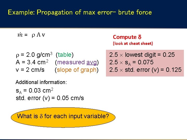
Example: Propagation of max error- brute force Compute (look at cheat sheet) = 2. 0 g/cm 3 (table) A = 3. 4 cm 2 (measured avg) v = 2 cm/s (slope of graph) Additional information: s. A = 0. 03 cm 2 std. error (v) = 0. 05 cm/s What is d for each input variable? 2. 5 lowest digit = 0. 25 2. 5 s. A = 0. 075 2. 5 std. error (v) = 0. 125

Example: Propagation of max error- brute force Brute force method: = 2. 0 A = 3. 4 cm 2 v = 2 cm/s g/cm 3 (table) (measured avg) (slope of graph) min max 1. 75 2. 25 A 3. 325 3. 475 v 1. 875 2. 125 Additional information: s. A = 0. 03 cm 2 std. error (v) = 0. 05 cm/s All combinations What is d for each input variable? 10. 9 16. 6 13. 6 3. 01 2. 69

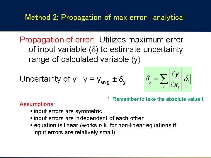
Method 2: Propagation of max error- analytical Propagation of error: Utilizes maximum error of input variable (d) to estimate uncertainty range of calculated variable (y) Uncertainty of y: y = yavg ± dy * Remember to take the absolute value!! Assumptions: • input errors are symmetric • input errors are independent of each other • equation is linear (works o. k. for non-linear equations if input errors are relatively small)

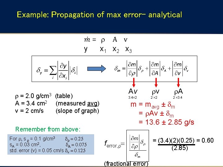
Example: Propagation of max error- analytical y = 2. 0 A = 3. 4 cm 2 v = 2 cm/s g/cm 3 x 1 x 2 x 3 Av (table) (measured avg) (slope of graph) 3. 4 2 2 2 A 2 3. 4 m = mavg ± dm = Av ± dm = 13. 6 ± 2. 85 g/s Remember from above: For , s = 0. 1 g/cm 3 d = 0. 25 s. A = 0. 03 cm 2, d. A = 0. 075 std. error (v) = 0. 05 cm/s dv = 0. 125 v ferror, = (fractional error) = (3. 4)(2)(0. 25) = 0. 60 (2. 85)

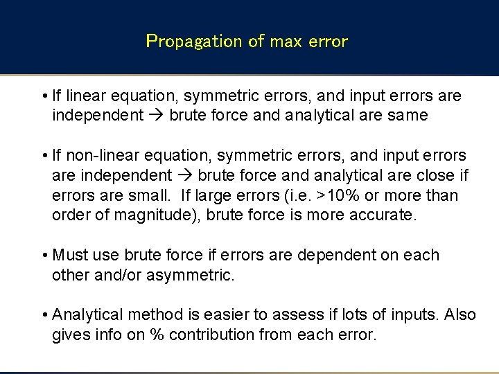
Propagation of max error • If linear equation, symmetric errors, and input errors are independent brute force and analytical are same • If non-linear equation, symmetric errors, and input errors are independent brute force and analytical are close if errors are small. If large errors (i. e. >10% or more than order of magnitude), brute force is more accurate. • Must use brute force if errors are dependent on each other and/or asymmetric. • Analytical method is easier to assess if lots of inputs. Also gives info on % contribution from each error.

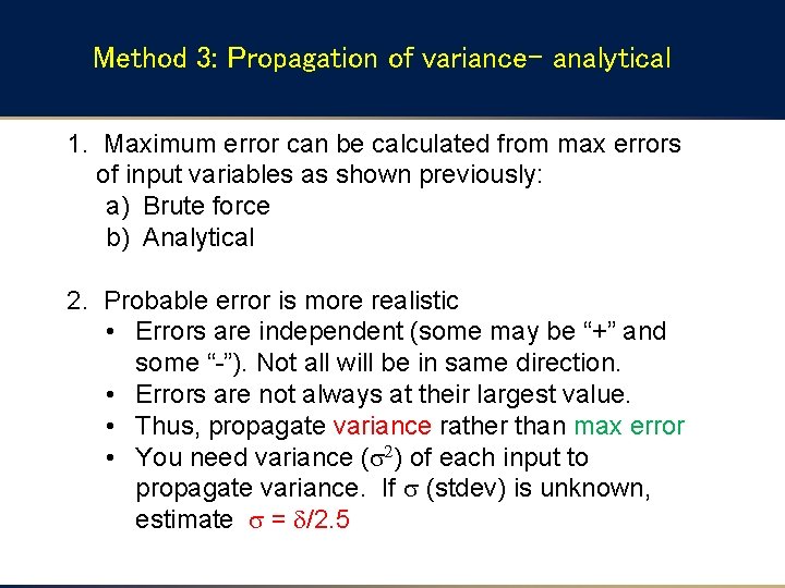
Method 3: Propagation of variance- analytical 1. Maximum error can be calculated from max errors of input variables as shown previously: a) Brute force b) Analytical 2. Probable error is more realistic • Errors are independent (some may be “+” and some “-”). Not all will be in same direction. • Errors are not always at their largest value. • Thus, propagate variance rather than max error • You need variance (s 2) of each input to propagate variance. If s (stdev) is unknown, estimate s = d/2. 5

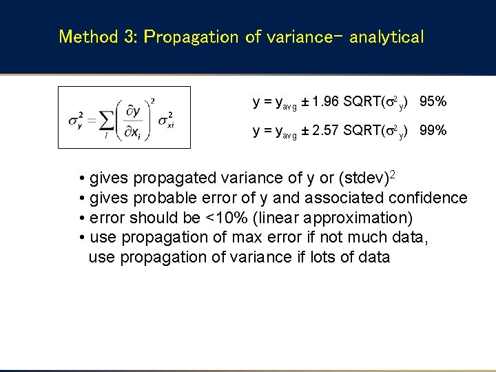
Method 3: Propagation of variance- analytical y = yavg ± 1. 96 SQRT(s 2 y) 95% y = yavg ± 2. 57 SQRT(s 2 y) 99% • gives propagated variance of y or (stdev)2 • gives probable error of y and associated confidence • error should be <10% (linear approximation) • use propagation of max error if not much data, use propagation of variance if lots of data

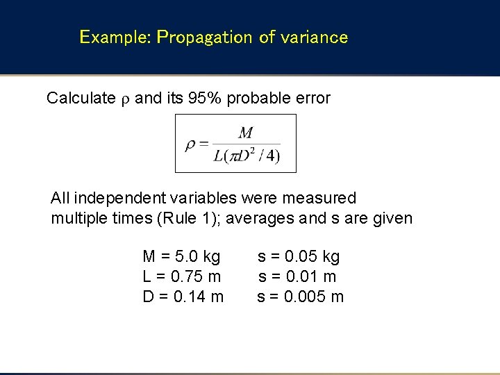
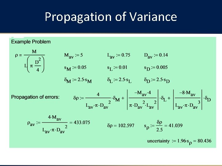
Example: Propagation of variance Calculate and its 95% probable error All independent variables were measured multiple times (Rule 1); averages and s are given M = 5. 0 kg L = 0. 75 m D = 0. 14 m s = 0. 05 kg s = 0. 01 m s = 0. 005 m

Propagation of Variance

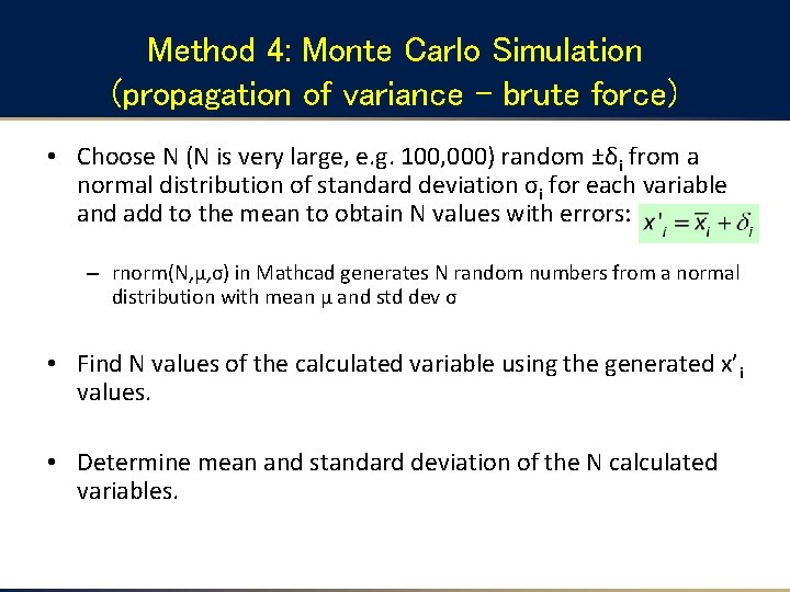
Method 4: Monte Carlo Simulation (propagation of variance – brute force) • Choose N (N is very large, e. g. 100, 000) random ±δi from a normal distribution of standard deviation σi for each variable and add to the mean to obtain N values with errors: – rnorm(N, μ, σ) in Mathcad generates N random numbers from a normal distribution with mean μ and std dev σ • Find N values of the calculated variable using the generated x’i values. • Determine mean and standard deviation of the N calculated variables.

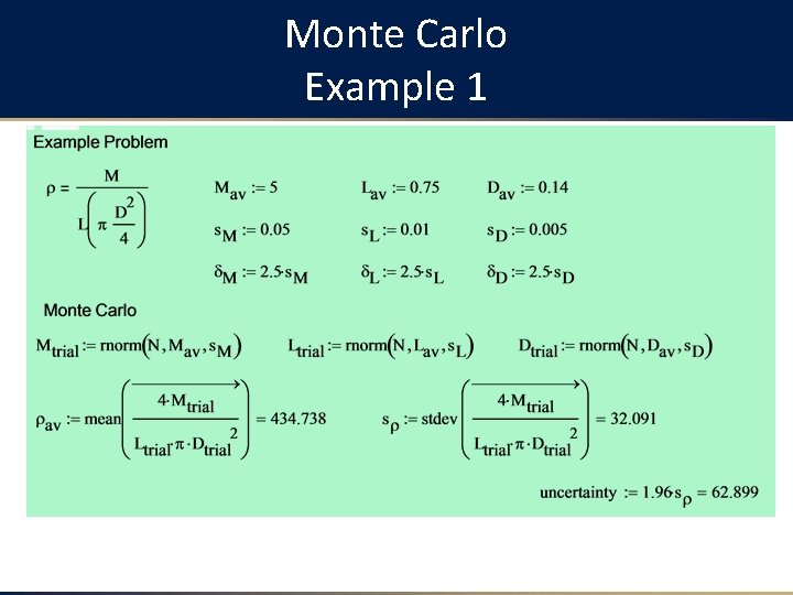
Monte Carlo Example 1

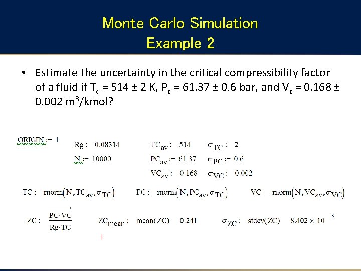
Monte Carlo Simulation Example 2 • Estimate the uncertainty in the critical compressibility factor of a fluid if Tc = 514 ± 2 K, Pc = 61. 37 ± 0. 6 bar, and Vc = 0. 168 ± 0. 002 m 3/kmol?

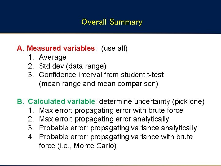
Overall Summary A. Measured variables: (use all) 1. Average 2. Std dev (data range) 3. Confidence interval from student t-test (mean range and mean comparison) B. Calculated variable: determine uncertainty (pick one) 1. Max error: propagating error with brute force 2. Max error: propagating error analytically 3. Probable error: propagating variance analytically 4. Probable error: propagating variance with brute force (i. e. , Monte Carlo)

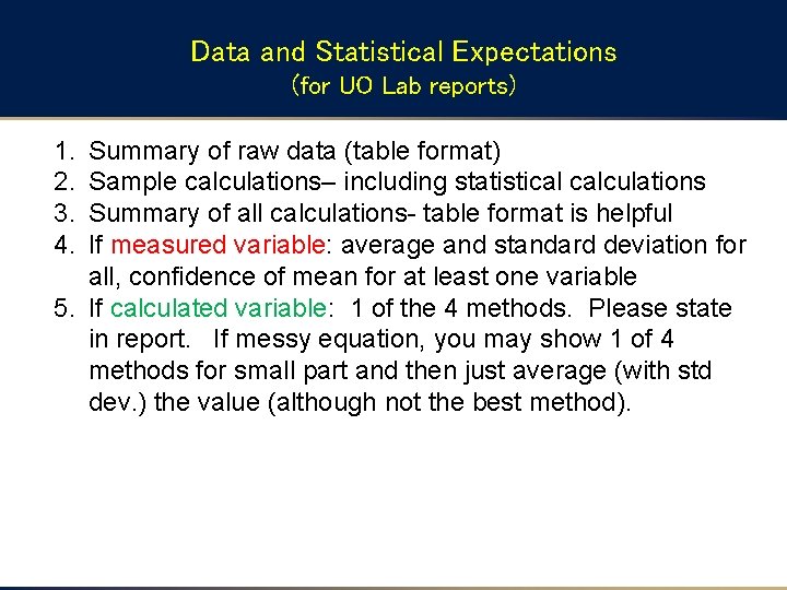
Data and Statistical Expectations (for UO Lab reports) 1. 2. 3. 4. Summary of raw data (table format) Sample calculations– including statistical calculations Summary of all calculations- table format is helpful If measured variable: average and standard deviation for all, confidence of mean for at least one variable 5. If calculated variable: 1 of the 4 methods. Please state in report. If messy equation, you may show 1 of 4 methods for small part and then just average (with std dev. ) the value (although not the best method).