Projecting Emissions Inventories for Air Quality Modeling of

Projecting Emissions Inventories for Air Quality Modeling of Future Years May 17, 2018 Alison Eyth, Jeff Vukovich, Caroline Farkas EPA Office of Air Quality Planning and Standards Emission Inventory and Analysis Group

Future Year Projections Course Outline and Schedule � 8: 30 Background Refresher � 9: 00 Introduction to projections � 9: 20 Control Strategy Tool overview � 9: 40 Agricultural and fugitive dust projections � 10: 00 Residential wood, commercial marine vessels, rail � 10: 15 Break � 10: 30 Oil and gas projections � 10: 55 Non. EGU point, Aviation � 11: 10 EGU � 11: 30 Onroad mobile source projections � 11: 45 Wrap up and final questions US EPA OAQPS, Emission Inventory and Analysis Group 2

Background: Purpose and Contents of a Modeling Platform � Air quality modeling platforms are used to support air quality studies ◦ Use technically sound data and state-of-the-science tools � Major ◦ ◦ ◦ components of a modeling platform: Meteorological models (WRF) and met. data Boundary conditions (GEOS-Chem/Hemispheric CMAQ) Emissions: base year (NEI)+Non. US, future year projections Air quality models (CMAQ, CAMx) Other: ancillary data for emissions modeling, projections data, emissions modeling tools (SMOKE, etc) and scripts US EPA OAQPS, Emission Inventory and Analysis Group 3

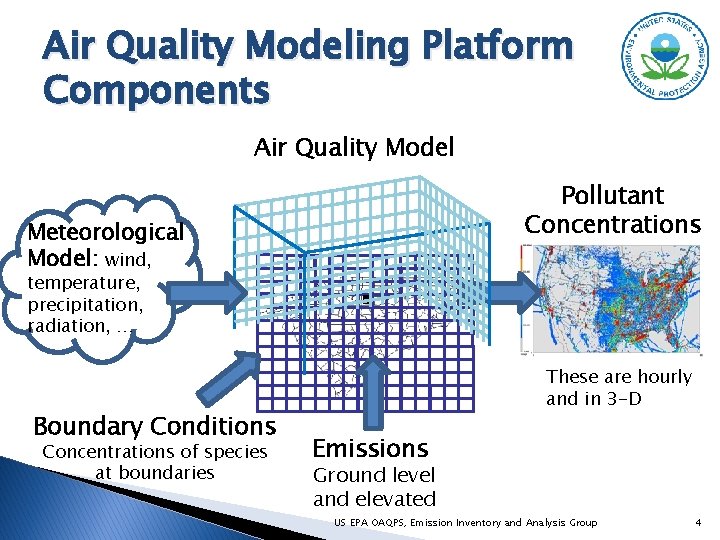
Air Quality Modeling Platform Components Air Quality Model Pollutant Concentrations Meteorological Model: wind, temperature, precipitation, radiation, … Boundary Conditions Concentrations of species at boundaries These are hourly and in 3 -D Emissions Ground level and elevated US EPA OAQPS, Emission Inventory and Analysis Group 4

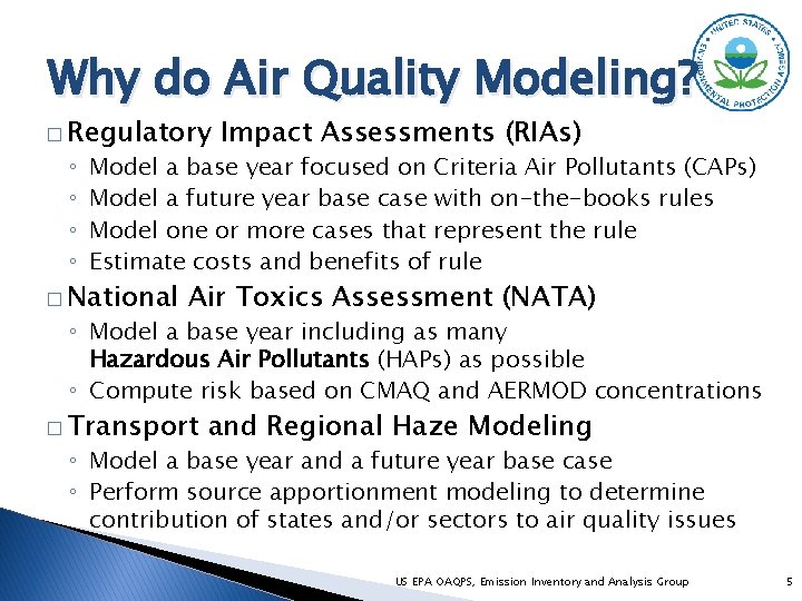
Why do Air Quality Modeling? � Regulatory ◦ ◦ Impact Assessments (RIAs) Model a base year focused on Criteria Air Pollutants (CAPs) Model a future year base case with on-the-books rules Model one or more cases that represent the rule Estimate costs and benefits of rule � National Air Toxics Assessment (NATA) ◦ Model a base year including as many Hazardous Air Pollutants (HAPs) as possible ◦ Compute risk based on CMAQ and AERMOD concentrations � Transport and Regional Haze Modeling ◦ Model a base year and a future year base case ◦ Perform source apportionment modeling to determine contribution of states and/or sectors to air quality issues US EPA OAQPS, Emission Inventory and Analysis Group 5

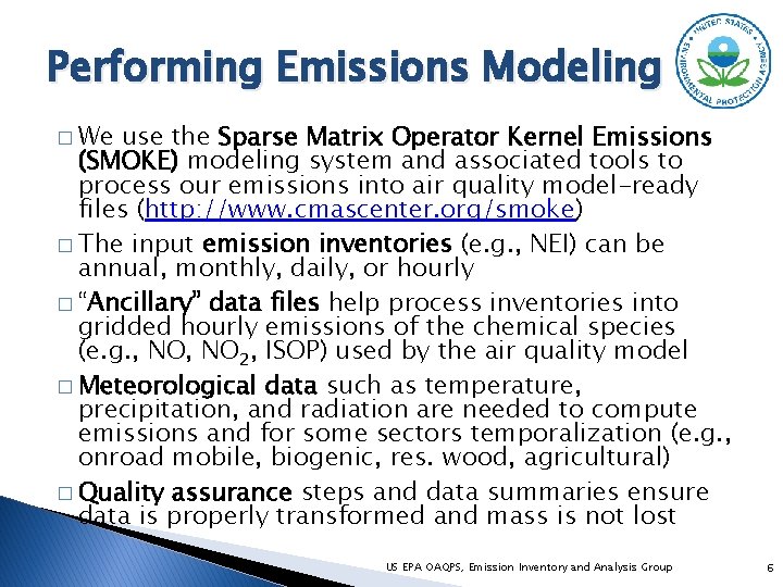
Performing Emissions Modeling � We use the Sparse Matrix Operator Kernel Emissions (SMOKE) modeling system and associated tools to process our emissions into air quality model-ready files (http: //www. cmascenter. org/smoke) � The input emission inventories (e. g. , NEI) can be annual, monthly, daily, or hourly � “Ancillary” data files help process inventories into gridded hourly emissions of the chemical species (e. g. , NO 2, ISOP) used by the air quality model � Meteorological data such as temperature, precipitation, and radiation are needed to compute emissions and for some sectors temporalization (e. g. , onroad mobile, biogenic, res. wood, agricultural) � Quality assurance steps and data summaries ensure data is properly transformed and mass is not lost US EPA OAQPS, Emission Inventory and Analysis Group 6

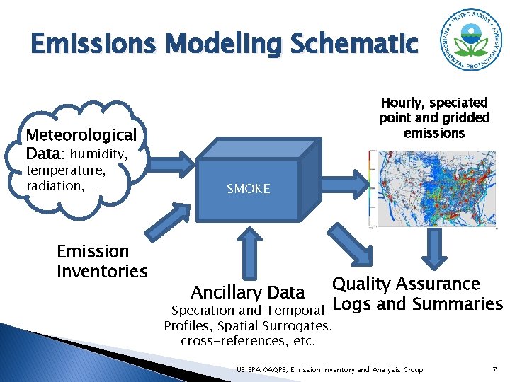
Emissions Modeling Schematic Hourly, speciated point and gridded emissions Meteorological Data: humidity, temperature, radiation, … Emission Inventories SMOKE Ancillary Data Quality Assurance Logs and Summaries Speciation and Temporal Profiles, Spatial Surrogates, cross-references, etc. US EPA OAQPS, Emission Inventory and Analysis Group 7

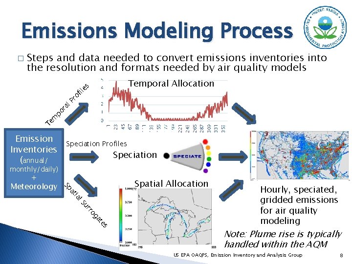
Emissions Modeling Process � Steps and data needed to convert emissions inventories into the resolution and formats needed by air quality models e fil ro P l Temporal Allocation s ra o p m Te Emission Inventories (annual/ Speciation Profiles Speciation monthly/daily) + Spatial Allocation l ia at Sp Meteorology es at og rr Su Hourly, speciated, gridded emissions for air quality modeling Note: Plume rise is typically handled within the AQM US EPA OAQPS, Emission Inventory and Analysis Group 8

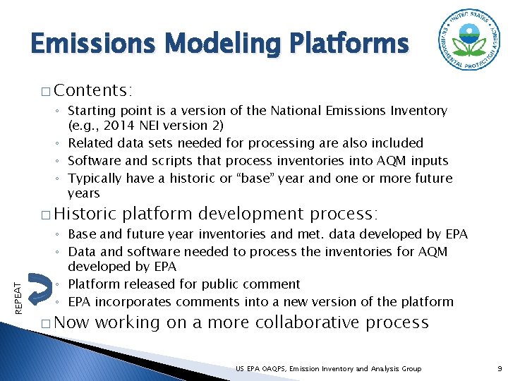
Emissions Modeling Platforms � Contents: ◦ Starting point is a version of the National Emissions Inventory (e. g. , 2014 NEI version 2) ◦ Related data sets needed for processing are also included ◦ Software and scripts that process inventories into AQM inputs ◦ Typically have a historic or “base” year and one or more future years REPEAT � Historic platform development process: ◦ Base and future year inventories and met. data developed by EPA ◦ Data and software needed to process the inventories for AQM developed by EPA ◦ Platform released for public comment ◦ EPA incorporates comments into a new version of the platform � Now working on a more collaborative process US EPA OAQPS, Emission Inventory and Analysis Group 9

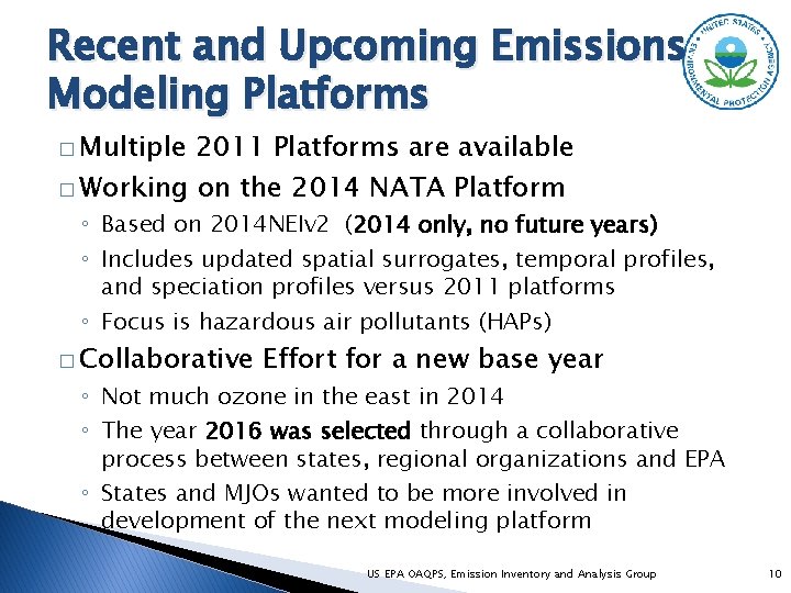
Recent and Upcoming Emissions Modeling Platforms � Multiple 2011 Platforms are available � Working on the 2014 NATA Platform ◦ Based on 2014 NEIv 2 (2014 only, no future years) ◦ Includes updated spatial surrogates, temporal profiles, and speciation profiles versus 2011 platforms ◦ Focus is hazardous air pollutants (HAPs) � Collaborative Effort for a new base year ◦ Not much ozone in the east in 2014 ◦ The year 2016 was selected through a collaborative process between states, regional organizations and EPA ◦ States and MJOs wanted to be more involved in development of the next modeling platform US EPA OAQPS, Emission Inventory and Analysis Group 10

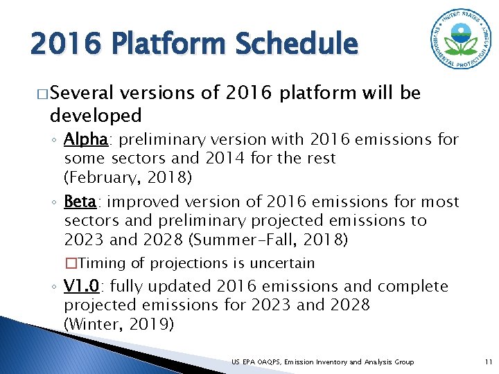
2016 Platform Schedule � Several versions of 2016 platform will be developed ◦ Alpha: preliminary version with 2016 emissions for some sectors and 2014 for the rest (February, 2018) ◦ Beta: improved version of 2016 emissions for most sectors and preliminary projected emissions to 2023 and 2028 (Summer-Fall, 2018) �Timing of projections is uncertain ◦ V 1. 0: fully updated 2016 emissions and complete projected emissions for 2023 and 2028 (Winter, 2019) US EPA OAQPS, Emission Inventory and Analysis Group 11

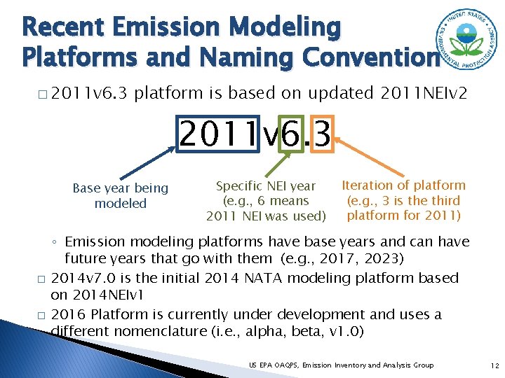
Recent Emission Modeling Platforms and Naming Convention � 2011 v 6. 3 platform is based on updated 2011 NEIv 2 2011 v 6. 3 Base year being modeled Specific NEI year (e. g. , 6 means 2011 NEI was used) Iteration of platform (e. g. , 3 is the third platform for 2011) ◦ Emission modeling platforms have base years and can have future years that go with them (e. g. , 2017, 2023) � 2014 v 7. 0 is the initial 2014 NATA modeling platform based on 2014 NEIv 1 � 2016 Platform is currently under development and uses a different nomenclature (i. e. , alpha, beta, v 1. 0) US EPA OAQPS, Emission Inventory and Analysis Group 12

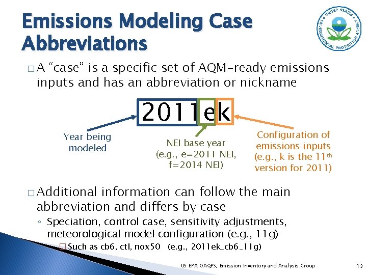
Emissions Modeling Case Abbreviations �A “case” is a specific set of AQM-ready emissions inputs and has an abbreviation or nickname Year being modeled 2011 ek NEI base year (e. g. , e=2011 NEI, f=2014 NEI) Configuration of emissions inputs (e. g. , k is the 11 th version for 2011) � Additional information can follow the main abbreviation and differs by case ◦ Speciation, control case, sensitivity adjustments, meteorological model configuration (e. g. , 11 g) � Such as cb 6, ctl, nox 50 (e. g. , 2011 ek_cb 6_11 g) US EPA OAQPS, Emission Inventory and Analysis Group 13

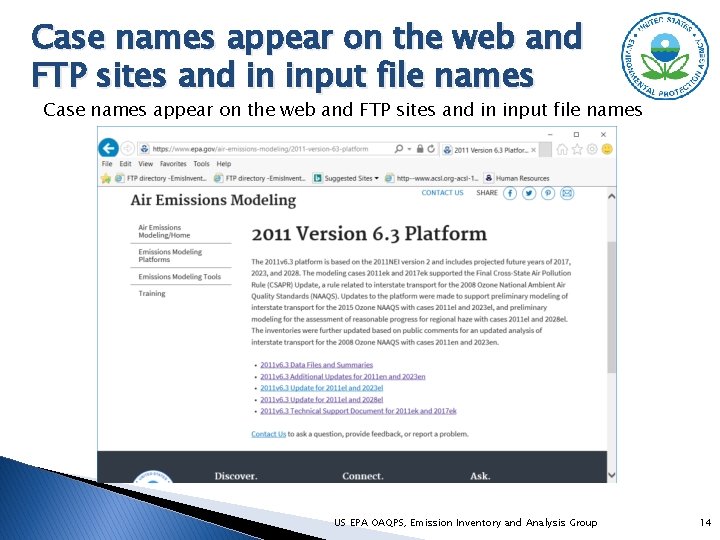
Case names appear on the web and FTP sites and in input file names US EPA OAQPS, Emission Inventory and Analysis Group 14

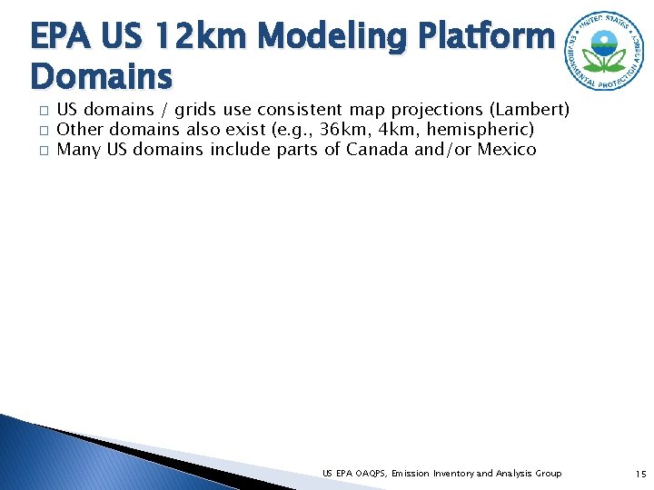
EPA US 12 km Modeling Platform Domains � � � US domains / grids use consistent map projections (Lambert) Other domains also exist (e. g. , 36 km, 4 km, hemispheric) Many US domains include parts of Canada and/or Mexico US EPA OAQPS, Emission Inventory and Analysis Group 15

Non-US emissions in the emissions modeling platform � Canada emissions & ancillary data (e. g. , surrogates) � Mexico 2008 emissions and projections of these ◦ Courtesy Environment Canada ◦ Used 2010 until 2013 and 2025 data provided in April, 2017 ◦ Fire emissions provided for summer 2011 and other years ◦ Based on Inventario Nacional de Emisiones de Mexico, 2008 ◦ MOVES-Mexico data was developed for key years ◦ Base year fire emissions for Mexico derived from Fire INventory from NCAR (FINN): � A daily fire emissions product for atmospheric chemistry models [also used for winter in Canada] � Hemispheric Transport of Air Pollution (HTAP) version 2 inventories used outside of North America in hemispheric runs US EPA OAQPS, Emission Inventory and Analysis Group 16

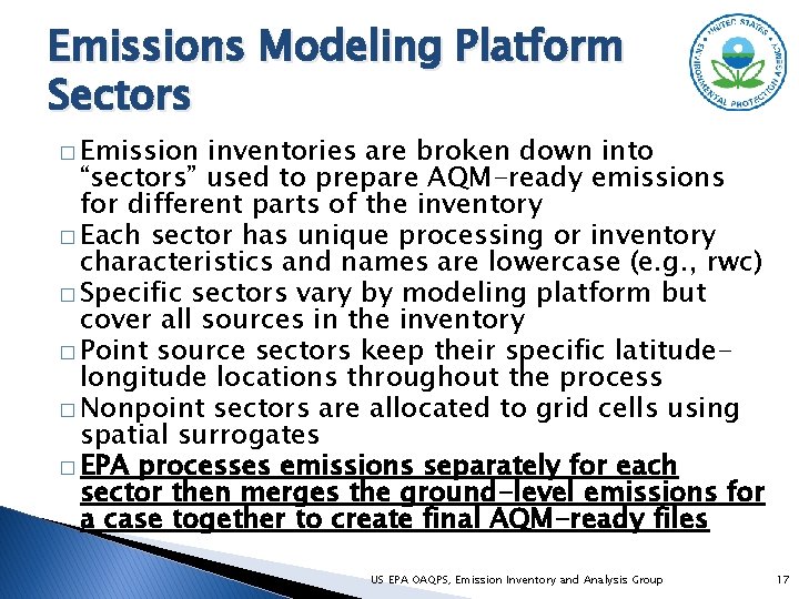
Emissions Modeling Platform Sectors � Emission inventories are broken down into “sectors” used to prepare AQM-ready emissions for different parts of the inventory � Each sector has unique processing or inventory characteristics and names are lowercase (e. g. , rwc) � Specific sectors vary by modeling platform but cover all sources in the inventory � Point source sectors keep their specific latitudelongitude locations throughout the process � Nonpoint sectors are allocated to grid cells using spatial surrogates � EPA processes emissions separately for each sector then merges the ground-level emissions for a case together to create final AQM-ready files US EPA OAQPS, Emission Inventory and Analysis Group 17

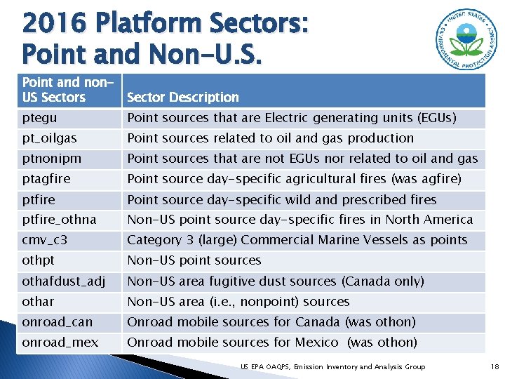
2016 Platform Sectors: Point and Non-U. S. Point and non. US Sectors Sector Description ptegu Point sources that are Electric generating units (EGUs) pt_oilgas Point sources related to oil and gas production ptnonipm Point sources that are not EGUs nor related to oil and gas ptagfire Point source day-specific agricultural fires (was agfire) ptfire Point source day-specific wild and prescribed fires ptfire_othna Non-US point source day-specific fires in North America cmv_c 3 Category 3 (large) Commercial Marine Vessels as points othpt Non-US point sources othafdust_adj Non-US area fugitive dust sources (Canada only) othar Non-US area (i. e. , nonpoint) sources onroad_can Onroad mobile sources for Canada (was othon) onroad_mex Onroad mobile sources for Mexico (was othon) US EPA OAQPS, Emission Inventory and Analysis Group 18

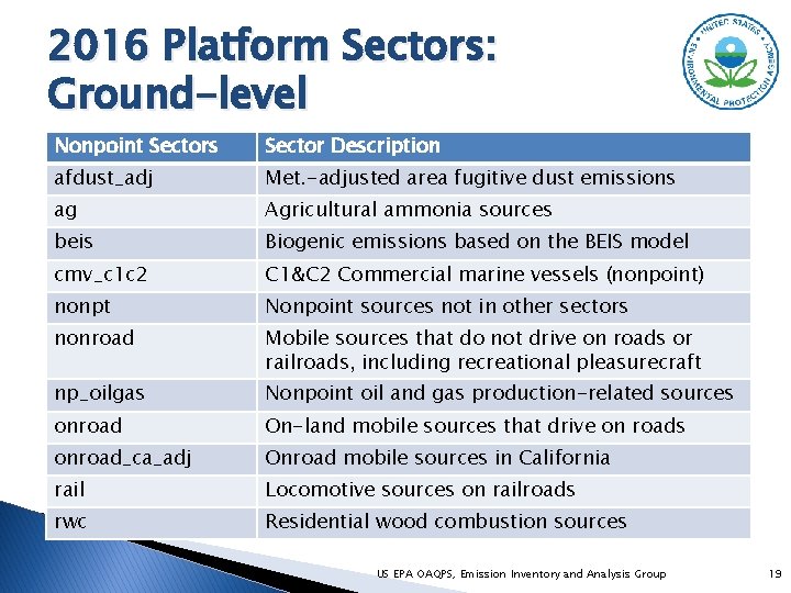
2016 Platform Sectors: Ground-level Nonpoint Sectors Sector Description afdust_adj Met. -adjusted area fugitive dust emissions ag Agricultural ammonia sources beis Biogenic emissions based on the BEIS model cmv_c 1 c 2 C 1&C 2 Commercial marine vessels (nonpoint) nonpt Nonpoint sources not in other sectors nonroad Mobile sources that do not drive on roads or railroads, including recreational pleasurecraft np_oilgas Nonpoint oil and gas production-related sources onroad On-land mobile sources that drive on roads onroad_ca_adj Onroad mobile sources in California rail Locomotive sources on railroads rwc Residential wood combustion sources US EPA OAQPS, Emission Inventory and Analysis Group 19

Questions? � Any questions on basic concepts of emissions modeling? US EPA OAQPS, Emission Inventory and Analysis Group 20

Course Outline and Schedule � 8: 30 Background Refresher � 9: 00 Introduction to projections � 9: 20 Control Strategy Tool overview � 9: 40 Agricultural and fugitive dust projections � 10: 00 Residential wood, commercial marine vessel, rail � 10: 15 Break � 10: 30 Oil and gas projections � 10: 55 Non. EGU point, Aviation � 11: 10 EGU � 11: 30 Onroad mobile source projections � 11: 45 Wrap up and final questions US EPA OAQPS, Emission Inventory and Analysis Group 21

Goals of Class � To introduce you to the various tasks involved with preparing emissions inputs to air quality models for future years ◦ Focus is on the steps and data involved, not the details of running the scripts � Note: presentation is available for download: ftp: //newftp. epa. gov/Air/nei/ei_training_may 2018/projecting_ei/ US EPA OAQPS, Emission Inventory and Analysis Group 22

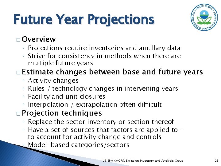
Future Year Projections � Overview ◦ Projections require inventories and ancillary data ◦ Strive for consistency in methods when there are multiple future years � Estimate ◦ ◦ changes between base and future years Activity changes Rules / technology changes in intervening years Facility and unit closures Interpolation / extrapolation often difficult � Projection techniques ◦ Replace the sector inventory or section thereof ◦ Have a set of sources that factors are applied to – to account for activity change and controls ◦ Model-based categories/sectors US EPA OAQPS, Emission Inventory and Analysis Group 23

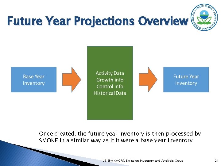
Future Year Projections Overview Once created, the future year inventory is then processed by SMOKE in a similar way as if it were a base year inventory US EPA OAQPS, Emission Inventory and Analysis Group 24

Why Develop Projected Emission Inventories? � Near-term projections ◦ The full NEI is developed every three years (2011, 2014, 2017, …) but we often need to do air quality modeling for years other than NEI years (e. g. , 2016) � Mid-term future projections (e. g. , through 2028) ◦ We need to evaluate policy options and impacts of changing emissions and use the results in a relative sense ◦ EPA develops Regulatory Impact Analyses (RIAs) for regulations �Describe the potential social benefits and social costs ◦ Interstate transport: The Clean Air Act’s "good neighbor" provision requires EPA and states to address interstate transport of air pollution that affects downwind states' ability to attain and maintain National Ambient Air Quality Standards (NAAQS) ◦ Other types of analyses US EPA OAQPS, Emission Inventory and Analysis Group 25

Developing Projections (1/2) � Future year emission inventories are developed starting with the base-year inventory and modeling platform ◦ Techniques vary by sector � For mid-term projections, base year-specific fires and biogenic emissions are typically also used in the future years US EPA OAQPS, Emission Inventory and Analysis Group 26

Developing Projections (2/2) � Factors to consider for each sector include: ◦ Confidence in base year inventory data ◦ Historical data available since base year ◦ What sources of information are available for each sector �Databases (e. g. Annual Energy Outlook (AEO)) �Models (e. g. Integrated Planning Model (IPM) for EGUs) ◦ How can these sources of information be used for estimating emissions? (e. g. , to update activity data) ◦ Spatial and temporal resolution of information ◦ Federal and state rules that go into effect in the intervening years are considered ◦ Point sources: consent decrees, planned shutdowns, etc. US EPA OAQPS, Emission Inventory and Analysis Group 27

Modeling Platforms with Projections � 2011 v 6. 3 platform ◦ https: //www. epa. gov/air-emissions-modeling/2011 -version 63 -platform ◦ Based on 2011 NEI version 2 with updates (used 5+ years) ◦ Originally supported the Final Cross-State Air Pollution Rule (CSAPR) Update with cases 2011 ek and 2017 ek, and 2017 ek_cntl ◦ Added 2011 el and 2023 el for a preliminary analysis of ozone transport with respect to the 2015 National Ambient Air Quality Standard (NAAQS) for ozone � 2011 en and 2023 en provided updates ◦ Added 2028 el for regional haze � Working towards projections based on 2014 NEI ◦ Need short-term (historical) projections to year 2016 ◦ Gathering data sources and information for mid-term US EPA OAQPS, Emission Inventory and Analysis Group 28

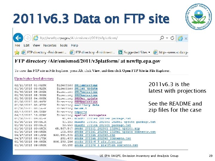
2011 v 6. 3 Data on FTP site 2011 v 6. 3 is the latest with projections See the README and zip files for the case US EPA OAQPS, Emission Inventory and Analysis Group 29

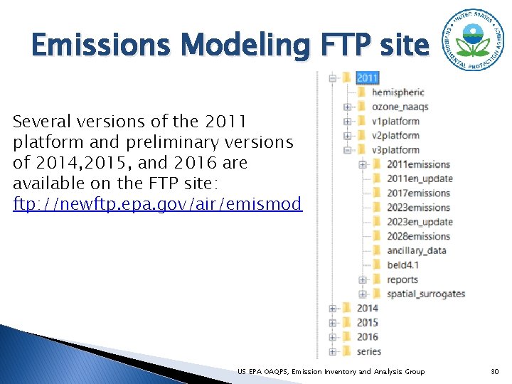
Emissions Modeling FTP site Several versions of the 2011 platform and preliminary versions of 2014, 2015, and 2016 are available on the FTP site: ftp: //newftp. epa. gov/air/emismod US EPA OAQPS, Emission Inventory and Analysis Group 30

Projection Techniques � Inventory projection techniques differ for different modeling platform sectors ◦ Some done using the Control Strategy Tool (Co. ST) within the Emissions Modeling Framework (EMF) ◦ Others are taken as outputs from models � Sparse Matrix Operator Kernel Emissions (SMOKE) modeling system is used to prepare the emissions for air quality models (e. g. CMAQ, CAMx) US EPA OAQPS, Emission Inventory and Analysis Group 31

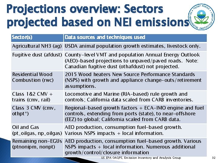
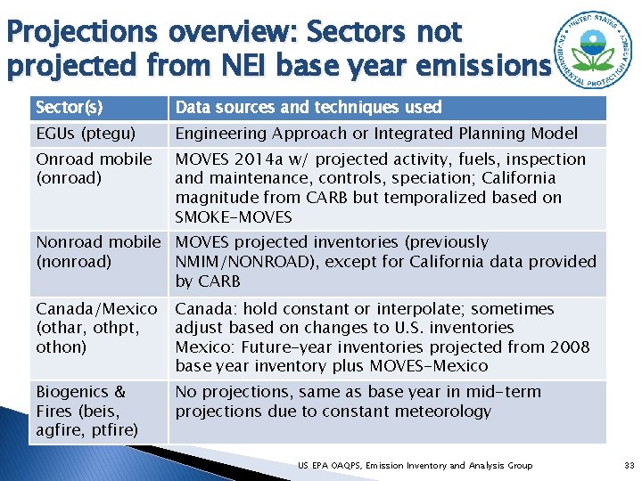
Projections overview: Sectors projected based on NEI emissions Sector(s) Data sources and techniques used Agricultural NH 3 (ag) USDA animal population growth estimates, livestock only. Fugitive dust (afdust) County-level VMT and population Annual Energy Outlook (AEO)-based projections to unpaved/paved roads. Note: Canadian fugitive dust (othafdust) not projected. Residential Wood Combustion (rwc) 2015 Wood heaters New Source Performance Standards (NSPS) with growth and appliance change-outs/retirement assumptions. Class 1&2 CMV + trains (cmv, rail) Locomotive and Marine (RIA-based) rule growth and controls; California data scaled from CARB inventories. Class 3 CMV (cmv, othpt*) Regional-based growth factors + ECA-IMO engine and fuel controls, extending from ports (state), to near-offshore (EEZ) to global; California scaled from CARB data. Oil and Gas AEO production, consumption fuel-based growth. (pt_oilgas, np_oilgas) Various NSPS impacts + local information. Remaining non-EGUs AEO production, consumption fuel-based growth. Various (ptnonipm, nonpt) NSPS impacts + local information. Numerous additional growth/control/closure information US EPA OAQPS, Emission Inventory and Analysis Group 32

Projections overview: Sectors not projected from NEI base year emissions Sector(s) Data sources and techniques used EGUs (ptegu) Engineering Approach or Integrated Planning Model Onroad mobile (onroad) MOVES 2014 a w/ projected activity, fuels, inspection and maintenance, controls, speciation; California magnitude from CARB but temporalized based on SMOKE-MOVES Nonroad mobile MOVES projected inventories (previously (nonroad) NMIM/NONROAD), except for California data provided by CARB Canada/Mexico (othar, othpt, othon) Canada: hold constant or interpolate; sometimes adjust based on changes to U. S. inventories Mexico: Future-year inventories projected from 2008 base year inventory plus MOVES-Mexico Biogenics & Fires (beis, agfire, ptfire) No projections, same as base year in mid-term projections due to constant meteorology US EPA OAQPS, Emission Inventory and Analysis Group 33

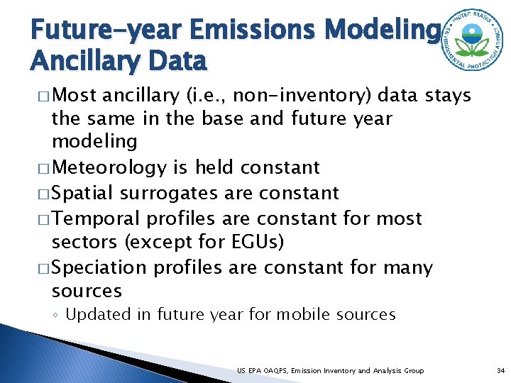
Future-year Emissions Modeling Ancillary Data � Most ancillary (i. e. , non-inventory) data stays the same in the base and future year modeling � Meteorology is held constant � Spatial surrogates are constant � Temporal profiles are constant for most sectors (except for EGUs) � Speciation profiles are constant for many sources ◦ Updated in future year for mobile sources US EPA OAQPS, Emission Inventory and Analysis Group 34

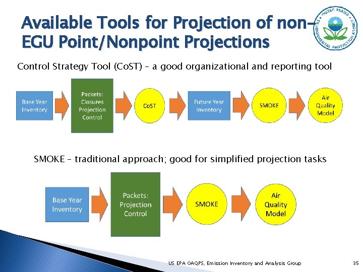
Available Tools for Projection of non. EGU Point/Nonpoint Projections Control Strategy Tool (Co. ST) – a good organizational and reporting tool SMOKE – traditional approach; good for simplified projection tasks US EPA OAQPS, Emission Inventory and Analysis Group 35

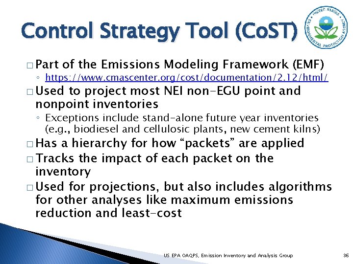
Control Strategy Tool (Co. ST) � Part of the Emissions Modeling Framework (EMF) ◦ https: //www. cmascenter. org/cost/documentation/2. 12/html/ � Used to project most NEI non-EGU point and nonpoint inventories ◦ Exceptions include stand-alone future year inventories (e. g. , biodiesel and cellulosic plants, new cement kilns) � Has a hierarchy for how “packets” are applied � Tracks the impact of each packet on the inventory � Used for projections, but also includes algorithms for other analyses like maximum emissions reduction and least-cost US EPA OAQPS, Emission Inventory and Analysis Group 36

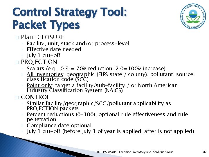
Control Strategy Tool: Packet Types � Plant CLOSURE � PROJECTION � CONTROL ◦ Facility, unit, stack and/or process-level ◦ Effective date needed ◦ July 1 cut-off ◦ Scalars (e. g. , 0. 3 = 70% reduction, 2. 0=100% increase) ◦ All inventories: geographic (FIPS state / county), pollutant, source classification code (SCC) ◦ Point only: target a facility/sub-facility / or North American Industry Classification System (NAICS) ◦ Similar facility/geographic/SCC/pollutant applicability as PROJECTION packets ◦ Percent reductions (0 -100), optional rule effectiveness and rule penetration ◦ Compliance date optional ◦ July 1 cut-off (before July 1 of year is applied, after is not applied) US EPA OAQPS, Emission Inventory and Analysis Group 37

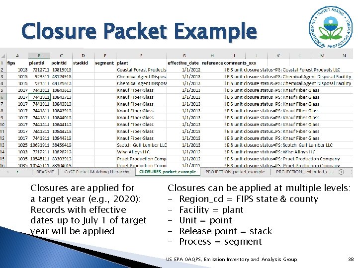
Closure Packet Example Closures are applied for a target year (e. g. , 2020): Records with effective dates up to July 1 of target year will be applied Closures can be applied at multiple levels: - Region_cd = FIPS state & county - Facility = plant - Unit = point - Release point = stack - Process = segment US EPA OAQPS, Emission Inventory and Analysis Group 38

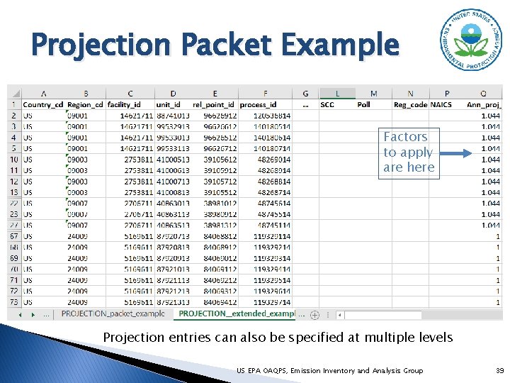
Projection Packet Example Factors to apply are here Projection entries can also be specified at multiple levels US EPA OAQPS, Emission Inventory and Analysis Group 39

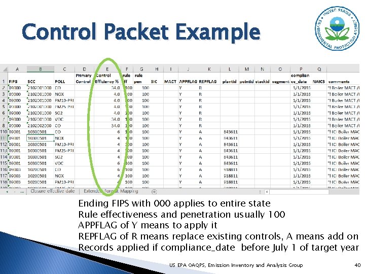
Control Packet Example Ending FIPS with 000 applies to entire state Rule effectiveness and penetration usually 100 APPFLAG of Y means to apply it REPFLAG of R means replace existing controls, A means add on Records applied if compliance_date before July 1 of target year US EPA OAQPS, Emission Inventory and Analysis Group 40

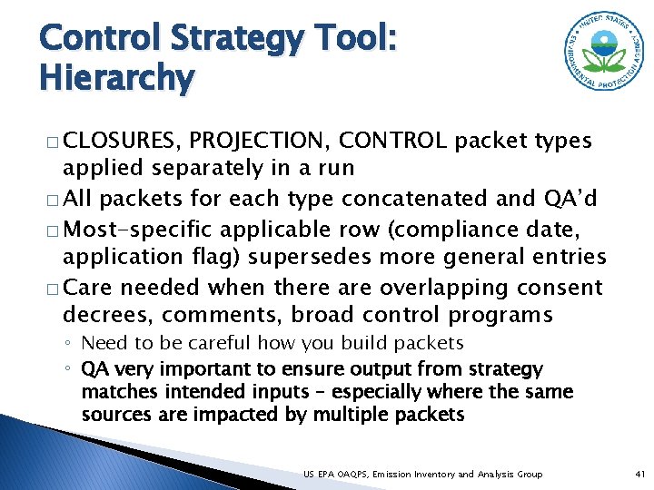
Control Strategy Tool: Hierarchy � CLOSURES, PROJECTION, CONTROL packet types applied separately in a run � All packets for each type concatenated and QA’d � Most-specific applicable row (compliance date, application flag) supersedes more general entries � Care needed when there are overlapping consent decrees, comments, broad control programs ◦ Need to be careful how you build packets ◦ QA very important to ensure output from strategy matches intended inputs – especially where the same sources are impacted by multiple packets US EPA OAQPS, Emission Inventory and Analysis Group 41

General -> Specific Co. ST Packet Priorities Entries in packets that are more specific have higher priority than the more general ones US EPA OAQPS, Emission Inventory and Analysis Group 42

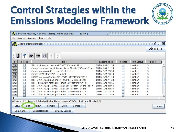
Control Strategies within the Emissions Modeling Framework US EPA OAQPS, Emission Inventory and Analysis Group 43

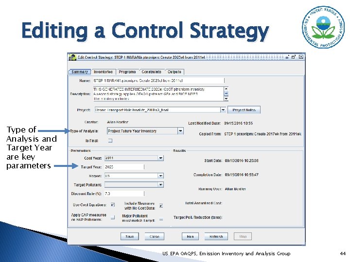
Editing a Control Strategy Type of Analysis and Target Year are key parameters US EPA OAQPS, Emission Inventory and Analysis Group 44

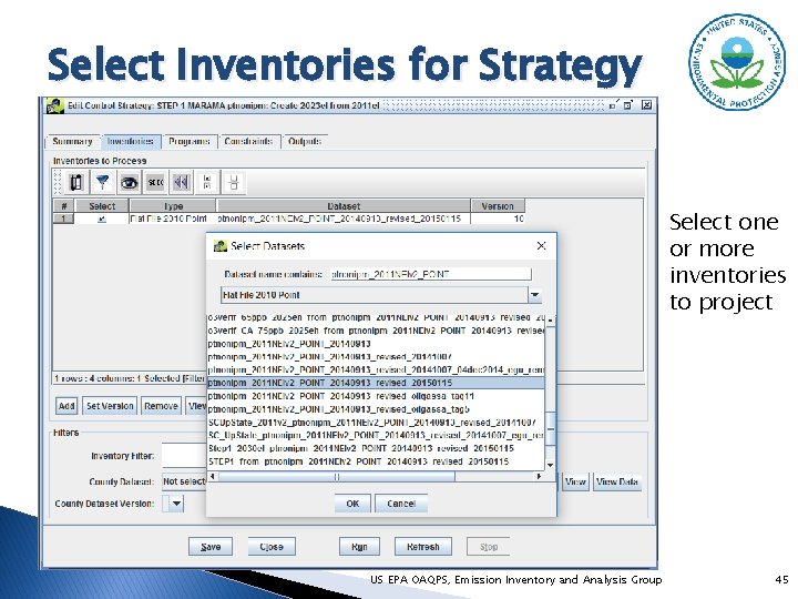
Select Inventories for Strategy Select one or more inventories to project US EPA OAQPS, Emission Inventory and Analysis Group 45

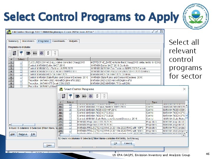
Select Control Programs to Apply Select all relevant control programs for sector US EPA OAQPS, Emission Inventory and Analysis Group 46

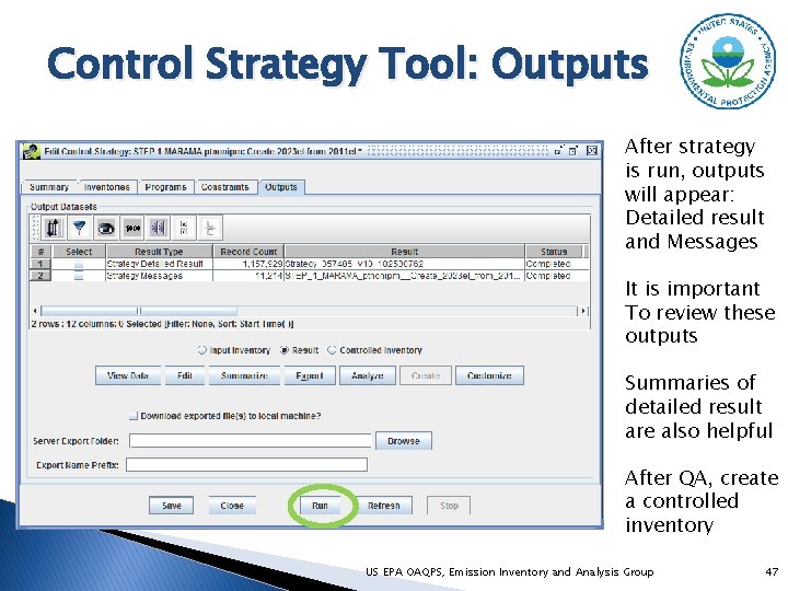
Control Strategy Tool: Outputs After strategy is run, outputs will appear: Detailed result and Messages It is important To review these outputs Summaries of detailed result are also helpful After QA, create a controlled inventory US EPA OAQPS, Emission Inventory and Analysis Group 47

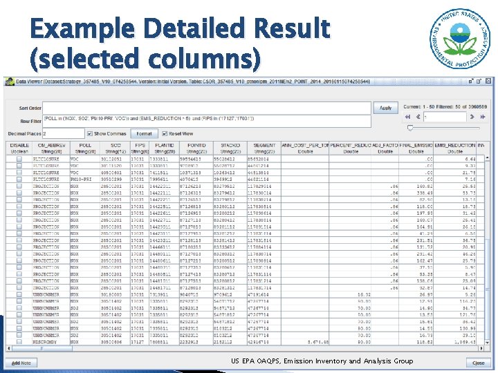
Example Detailed Result (selected columns) US EPA OAQPS, Emission Inventory and Analysis Group 48

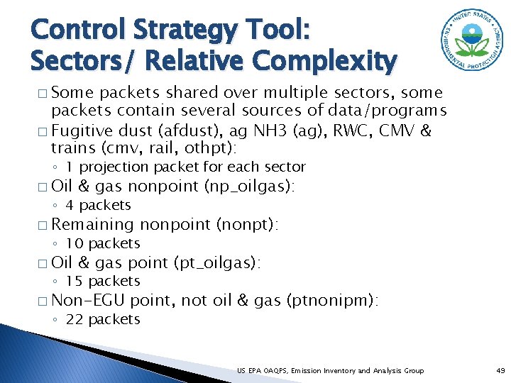
Control Strategy Tool: Sectors/ Relative Complexity � Some packets shared over multiple sectors, some packets contain several sources of data/programs � Fugitive dust (afdust), ag NH 3 (ag), RWC, CMV & trains (cmv, rail, othpt): ◦ 1 projection packet for each sector � Oil & gas nonpoint (np_oilgas): ◦ 4 packets � Remaining nonpoint (nonpt): ◦ 10 packets � Oil & gas point (pt_oilgas): ◦ 15 packets � Non-EGU point, not oil & gas (ptnonipm): ◦ 22 packets US EPA OAQPS, Emission Inventory and Analysis Group 49

Projections: Quality Assurance � Co. ST detailed summaries � Numerous template options in EMF for Structured Query Language (SQL)-based QA reports ◦ ◦ ◦ By control program Geography (e. g. , state, county) Source classification code (SCC) Can limit pollutants in summary Option to show “unaffected” sources � Can also create custom reports and summaries � Co. ST filter/sorts, export to CSV US EPA OAQPS, Emission Inventory and Analysis Group 50

Questions? � Any questions on the Control Strategy Tool? US EPA OAQPS, Emission Inventory and Analysis Group 51

Nonpoint Projections US EPA OAQPS, Emission Inventory and Analysis Group 52

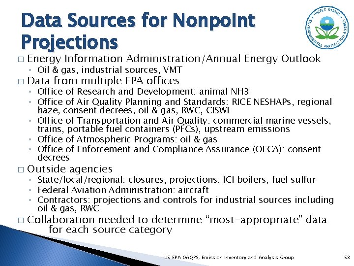
Data Sources for Nonpoint Projections � Energy Information Administration/Annual Energy Outlook � Data from multiple EPA offices � Outside agencies � ◦ Oil & gas, industrial sources, VMT ◦ Office of Research and Development: animal NH 3 ◦ Office of Air Quality Planning and Standards: RICE NESHAPs, regional haze, consent decrees, oil & gas, RWC, CISWI ◦ Office of Transportation and Air Quality: commercial marine vessels, trains, portable fuel containers (PFCs), upstream emissions ◦ Office of Atmospheric Programs: oil & gas ◦ Office of Enforcement and Compliance Assurance (OECA): consent decrees ◦ State/local/regional: closures, projections, ICI boilers, fuel sulfur ◦ Federal Aviation Administration: aircraft ◦ Contractors: projections and controls for industrial sources including oil & gas, RWC Collaboration needed to determine “most-appropriate” data for each source category US EPA OAQPS, Emission Inventory and Analysis Group 53

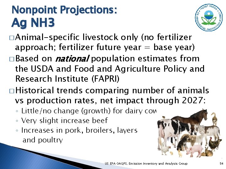
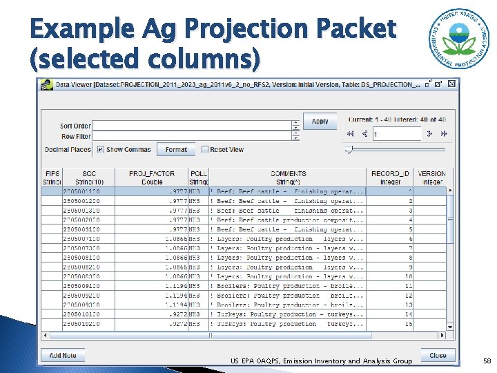
Nonpoint Projections: Ag NH 3 � Animal-specific livestock only (no fertilizer approach; fertilizer future year = base year) � Based on national population estimates from the USDA and Food and Agriculture Policy and Research Institute (FAPRI) � Historical trends comparing number of animals vs production rates, net impact through 2027: ◦ Little/no change (growth) for dairy cows, turkey ◦ Very slight increase beef ◦ Increases in pork, broilers, layers and poultry US EPA OAQPS, Emission Inventory and Analysis Group 54

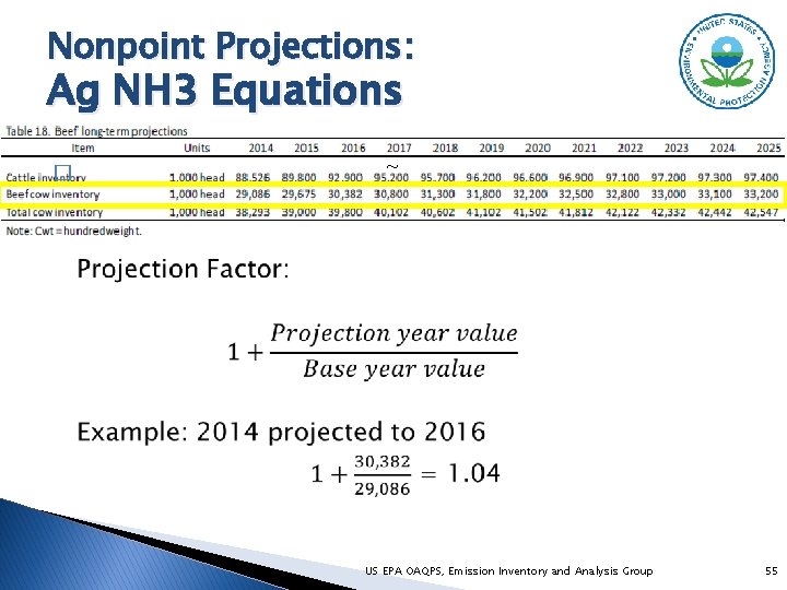
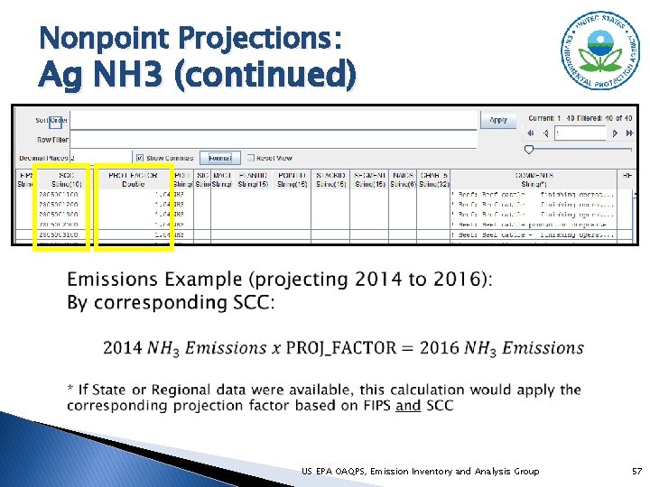
Nonpoint Projections: Ag NH 3 Equations � ~ US EPA OAQPS, Emission Inventory and Analysis Group 55

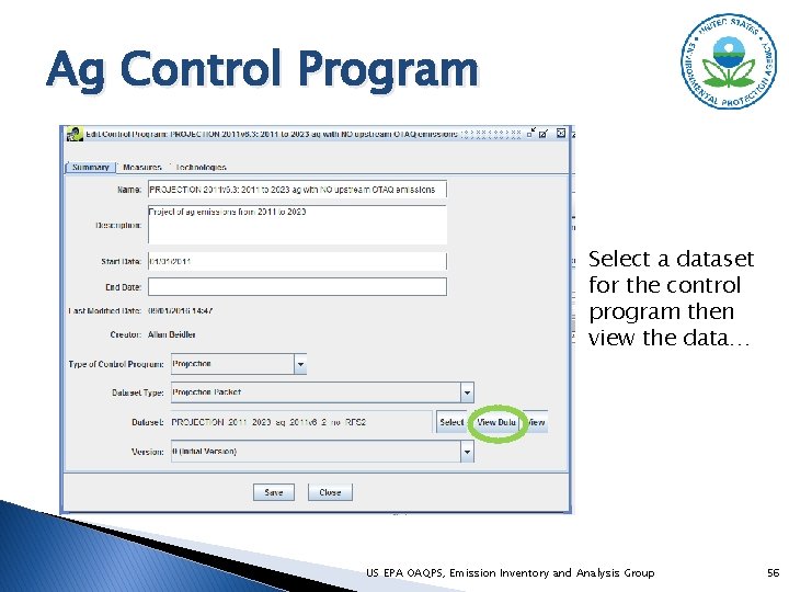
Ag Control Program Select a dataset for the control program then view the data… US EPA OAQPS, Emission Inventory and Analysis Group 56

Nonpoint Projections: Ag NH 3 (continued) � US EPA OAQPS, Emission Inventory and Analysis Group 57

Example Ag Projection Packet (selected columns) US EPA OAQPS, Emission Inventory and Analysis Group 58

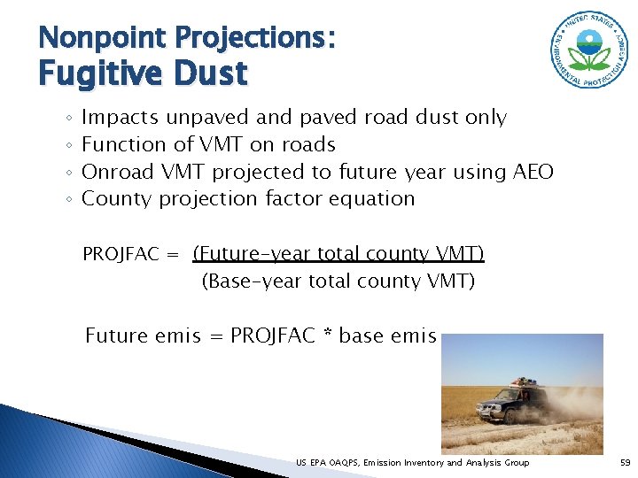
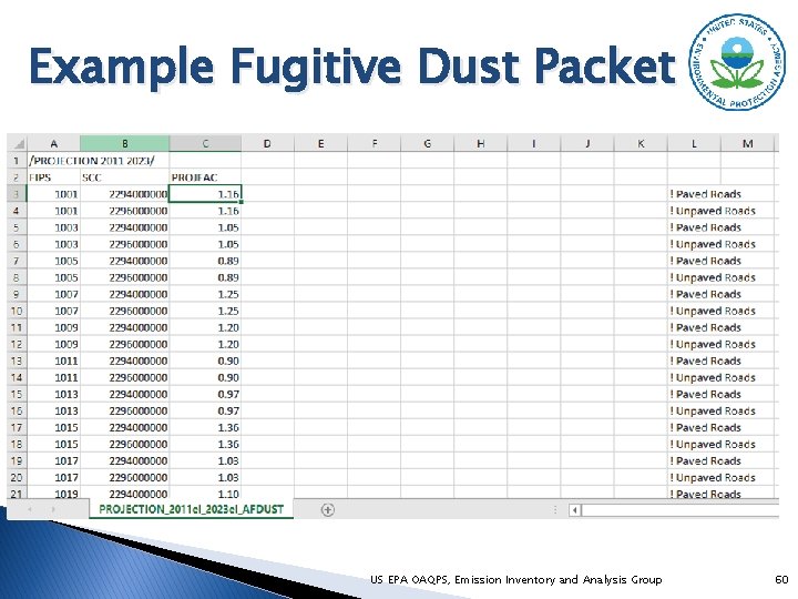
Nonpoint Projections: Fugitive Dust ◦ ◦ Impacts unpaved and paved road dust only Function of VMT on roads Onroad VMT projected to future year using AEO County projection factor equation PROJFAC = (Future-year total county VMT) (Base-year total county VMT) Future emis = PROJFAC * base emis US EPA OAQPS, Emission Inventory and Analysis Group 59

Example Fugitive Dust Packet US EPA OAQPS, Emission Inventory and Analysis Group 60

QA of ag/afdust Projections � Compare base and future year emissions to ensure that factors were properly applied � Create percent and absolute difference maps to make sure that results are as expected � Note: Future year fugitive dust inventories undergo meteorological and transport fraction reductions like the base year ones do US EPA OAQPS, Emission Inventory and Analysis Group 61

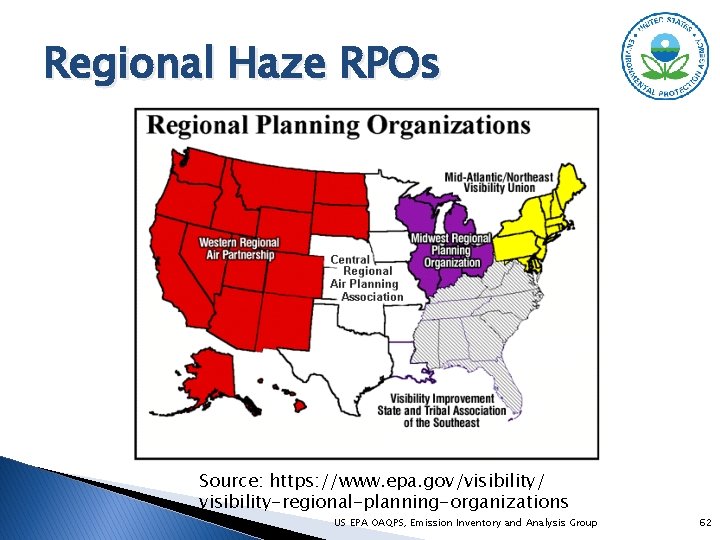
Regional Haze RPOs Source: https: //www. epa. gov/visibility/ visibility-regional-planning-organizations US EPA OAQPS, Emission Inventory and Analysis Group 62

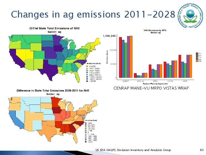
Changes in ag emissions 2011 -2028 1, 500, 000 CENRAP MANE-VU MRPO VISTAS WRAP US EPA OAQPS, Emission Inventory and Analysis Group 63

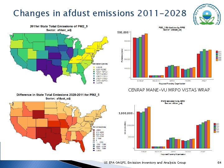
Changes in afdust emissions 2011 -2028 500, 000 CENRAP MANE-VU MRPO VISTAS WRAP 3, 000 US EPA OAQPS, Emission Inventory and Analysis Group 64

Questions? � Any questions on ag or fugitive dust projections? US EPA OAQPS, Emission Inventory and Analysis Group 65

Nonpoint Projections: Residential Wood Combustion Growth derived from year 2012 appliance shipments and forecast revenue forecasts (e. g. US Bureau of Economic Analysis) � Updated to include recently promulgated NSPS for ‘wood heaters’: http: //www 2. epa. gov/residential-wood-heaters/final-new-source� performance-standards-residential-wood-heaters Net decrease rather than increase in RWC emissions vs business as usual approach in prior platform � Reflect year 2015 rulemaking and minor corrections � Appliance-specific retirement/replacement rates for most sources � “No-change” assumption used in western states: WA, OR, CA � Burn bans not addressed in 2011 platforms � US EPA OAQPS, Emission Inventory and Analysis Group 66

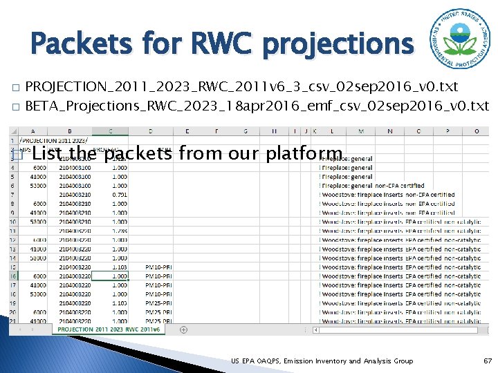
Packets for RWC projections � � � PROJECTION_2011_2023_RWC_2011 v 6_3_csv_02 sep 2016_v 0. txt BETA_Projections_RWC_2023_18 apr 2016_emf_csv_02 sep 2016_v 0. txt List the packets from our platform US EPA OAQPS, Emission Inventory and Analysis Group 67

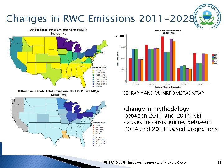
Changes in RWC Emissions 2011 -2028 120, 000 CENRAP MANE-VU MRPO VISTAS WRAP Change in methodology between 2011 and 2014 NEI causes inconsistencies between 2014 and 2011 -based projections US EPA OAQPS, Emission Inventory and Analysis Group 68

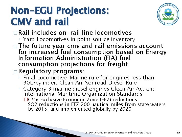
Non-EGU Projections: CMV and rail � Rail includes on-rail line locomotives ◦ Yard Locomotives in point source inventory � The future year cmv and rail emissions account for increased fuel consumption based on Energy Information Administration (EIA) fuel consumption projections for freight � Regulatory programs: ◦ Final Locomotive-Marine rule for engines less than 30 L/cylinder, Clean Air Nonroad Diesel Rule ◦ Category 3 marine diesel engines Clean Air Act and International Maritime Organization Standards �CMV Exclusive Economic Zone (EEZ) reductions: SO 2 reductions in EEZ 200 nautical miles from state waters by 2015, and implemented globally by 2020 US EPA OAQPS, Emission Inventory and Analysis Group 69

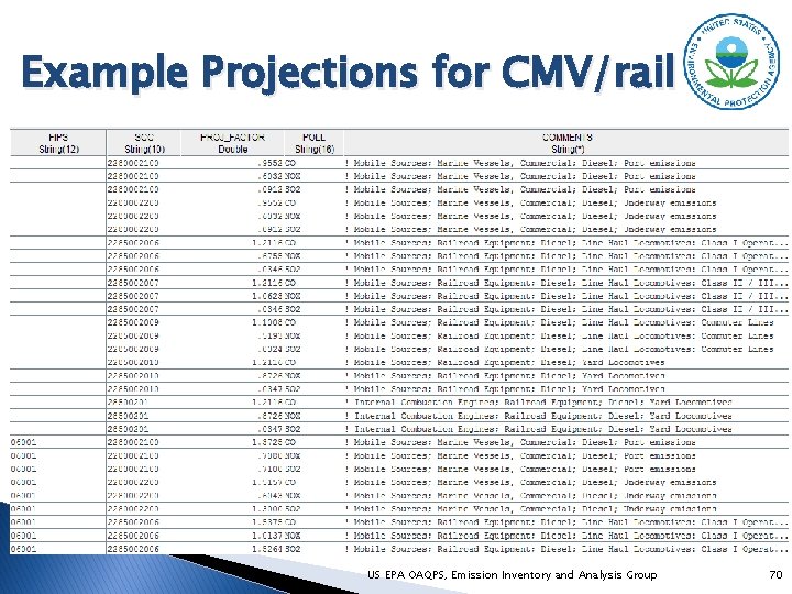
Example Projections for CMV/rail US EPA OAQPS, Emission Inventory and Analysis Group 70

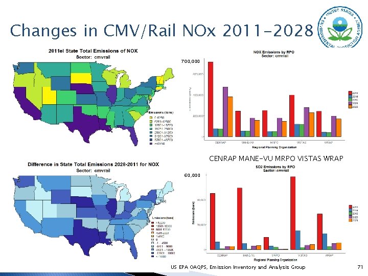
Changes in CMV/Rail NOx 2011 -2028 700, 000 CENRAP MANE-VU MRPO VISTAS WRAP 60, 000 US EPA OAQPS, Emission Inventory and Analysis Group 71

Questions? � Any questions on RWC, CMV, or rail projections? US EPA OAQPS, Emission Inventory and Analysis Group 72

Oil and Gas Projections � Volatile sector; growth changing frequently � Various approaches ◦ Pros and cons of each � Various data sources ◦ State historical data ◦ AEO publicly available tables ◦ AEO internal tables (EIA) US EPA OAQPS, Emission Inventory and Analysis Group 73

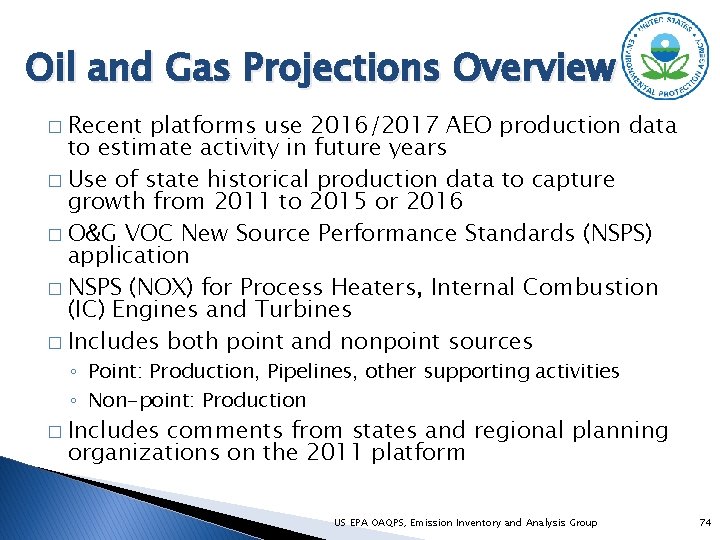
Oil and Gas Projections Overview � Recent platforms use 2016/2017 AEO production data to estimate activity in future years � Use of state historical production data to capture growth from 2011 to 2015 or 2016 � O&G VOC New Source Performance Standards (NSPS) application � NSPS (NOX) for Process Heaters, Internal Combustion (IC) Engines and Turbines � Includes both point and nonpoint sources ◦ Point: Production, Pipelines, other supporting activities ◦ Non-point: Production � Includes comments from states and regional planning organizations on the 2011 platform US EPA OAQPS, Emission Inventory and Analysis Group 74

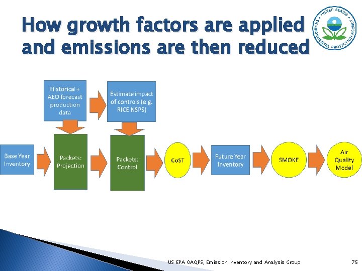
How growth factors are applied and emissions are then reduced US EPA OAQPS, Emission Inventory and Analysis Group 75

Oil and Gas Projections: Basin level production forecasts from 2011 v 6. 2 US EPA OAQPS, Emission Inventory and Analysis Group 76

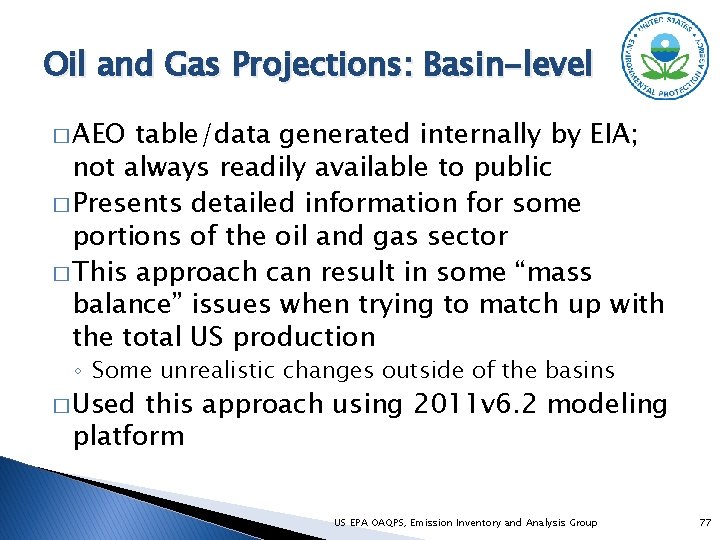
Oil and Gas Projections: Basin-level � AEO table/data generated internally by EIA; not always readily available to public � Presents detailed information for some portions of the oil and gas sector � This approach can result in some “mass balance” issues when trying to match up with the total US production ◦ Some unrealistic changes outside of the basins � Used this approach using 2011 v 6. 2 modeling platform US EPA OAQPS, Emission Inventory and Analysis Group 77

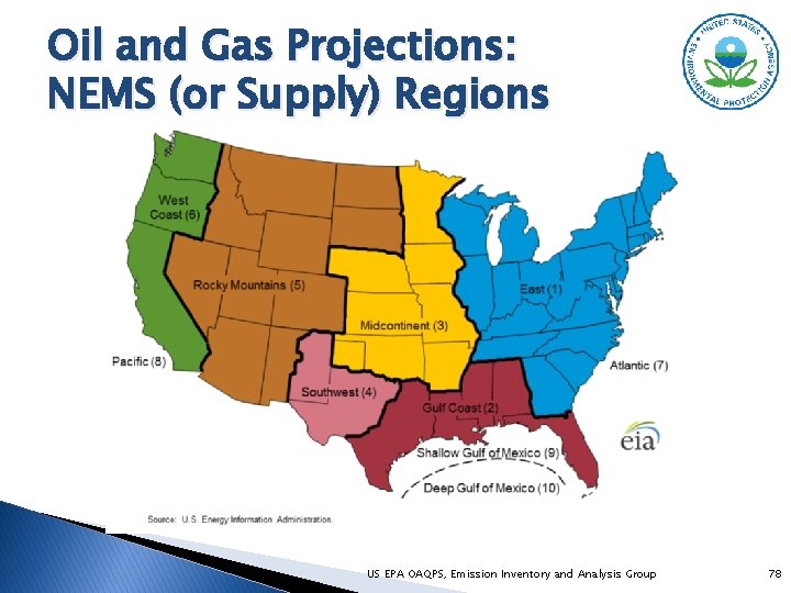
Oil and Gas Projections: NEMS (or Supply) Regions US EPA OAQPS, Emission Inventory and Analysis Group 78

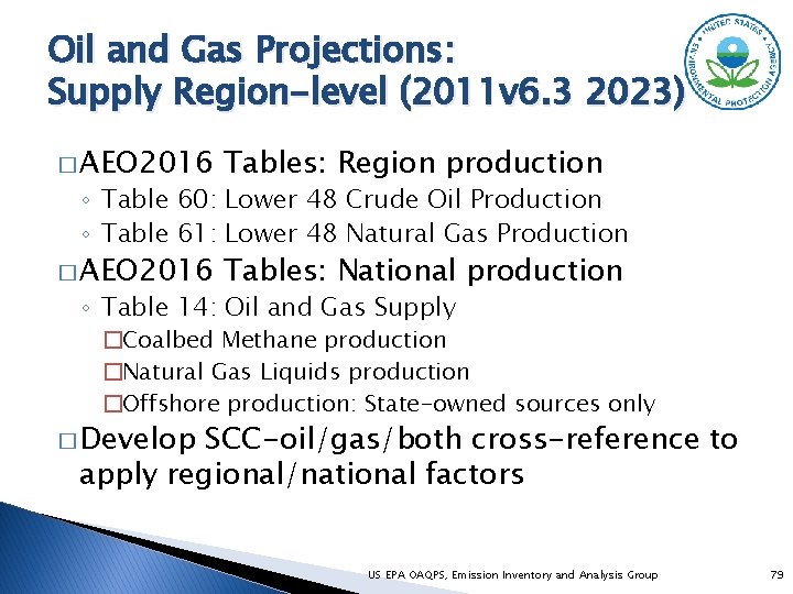
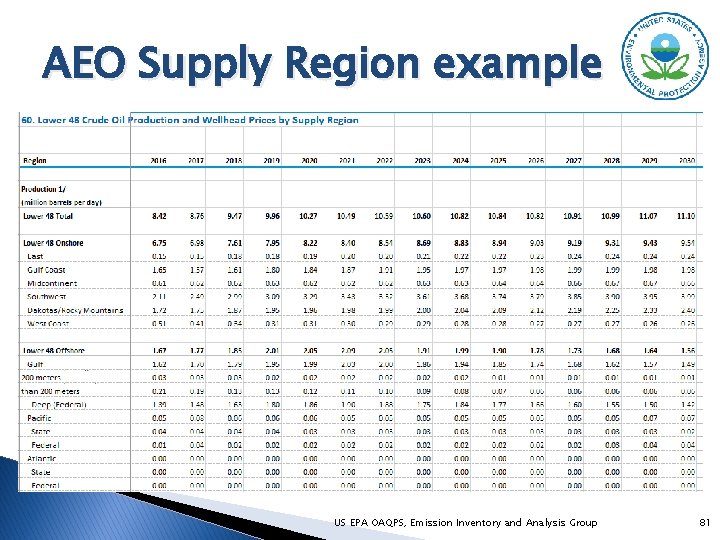
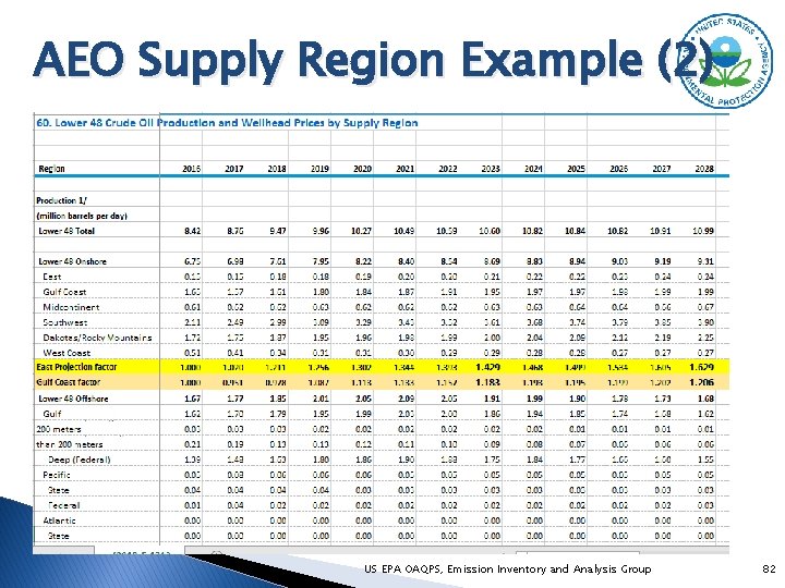
Oil and Gas Projections: Supply Region-level (2011 v 6. 3 2023) � AEO 2016 Tables: Region production � AEO 2016 Tables: National production ◦ Table 60: Lower 48 Crude Oil Production ◦ Table 61: Lower 48 Natural Gas Production ◦ Table 14: Oil and Gas Supply �Coalbed Methane production �Natural Gas Liquids production �Offshore production: State-owned sources only � Develop SCC-oil/gas/both cross-reference to apply regional/national factors US EPA OAQPS, Emission Inventory and Analysis Group 79

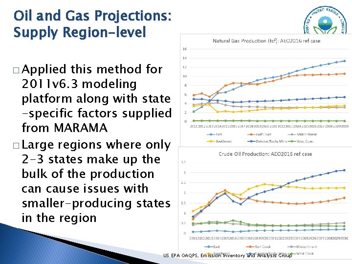
Oil and Gas Projections: Supply Region-level � Applied this method for 2011 v 6. 3 modeling platform along with state -specific factors supplied from MARAMA � Large regions where only 2 -3 states make up the bulk of the production cause issues with smaller-producing states in the region US EPA OAQPS, Emission Inventory and Analysis Group 80

AEO Supply Region example US EPA OAQPS, Emission Inventory and Analysis Group 81

AEO Supply Region Example (2) US EPA OAQPS, Emission Inventory and Analysis Group 82

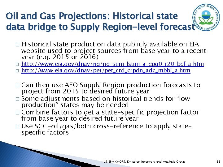
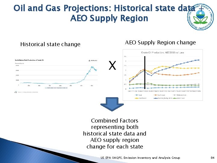
Oil and Gas Projections: Historical state data bridge to Supply Region-level forecast � � � Historical state production data publicly available on EIA website used to project sources from base year to a recent year (e. g. 2015 or 2016) http: //www. eia. gov/dnav/ng/ng_sum_lsum_a_epg 0_r 20_bcf_a. htm http: //www. eia. gov/dnav/pet_crd_crpdn_adc_mbbl_a. htm Can then use AEO Supply Region production forecasts to project from 2015 to desired future year � Some adjustments based on historical trends for “low production” states may be needed � Combine factors to get a state-specific projection factor from base year to desired future year � Use SCC-oil/gas/both cross-reference to apply statespecific factors � US EPA OAQPS, Emission Inventory and Analysis Group 83

Oil and Gas Projections: Historical state data + AEO Supply Region change Historical state change X Combined Factors representing both historical state data and AEO supply region change for each state US EPA OAQPS, Emission Inventory and Analysis Group 84

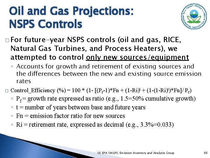
Oil and Gas Projections: NSPS Controls � For future-year NSPS controls (oil and gas, RICE, Natural Gas Turbines, and Process Heaters), we attempted to control only new sources/equipment ◦ Accounts for growth and retirement of existing sources and the differences between the new and existing source emission rates � Control_Efficiency (%) = 100 * (1 - [(Pf-1)*Fn + (1 -Ri)t + (1 -(1 -Ri)t)*Fn]/ Pf) ◦ ◦ Pf = growth rate expressed as ratio (e. g. , 1. 5=50% cumulative growth) t = number of years between base and future years Fn = emission factor ratio for new sources Ri = retirement rate, expressed as decimal (e. g. , 3. 3%=0. 033) US EPA OAQPS, Emission Inventory and Analysis Group 85

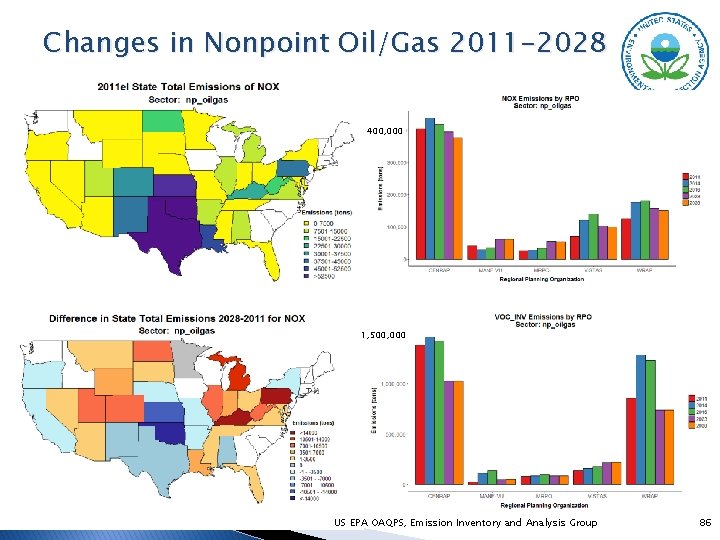
Changes in Nonpoint Oil/Gas 2011 -2028 400, 000 1, 500, 000 US EPA OAQPS, Emission Inventory and Analysis Group 86

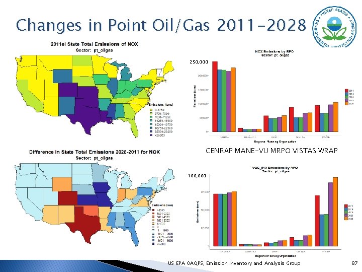
Changes in Point Oil/Gas 2011 -2028 250, 000 CENRAP MANE-VU MRPO VISTAS WRAP 100, 000 US EPA OAQPS, Emission Inventory and Analysis Group 87

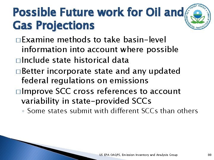
Possible Future work for Oil and Gas Projections � Examine methods to take basin-level information into account where possible � Include state historical data � Better incorporate state and any updated federal regulations on emissions � Improve SCC cross references to account variability in state-provided SCCs ◦ Some states submit with different SCCs than others US EPA OAQPS, Emission Inventory and Analysis Group 88

Questions on Oil and Gas Projections? US EPA OAQPS, Emission Inventory and Analysis Group 89

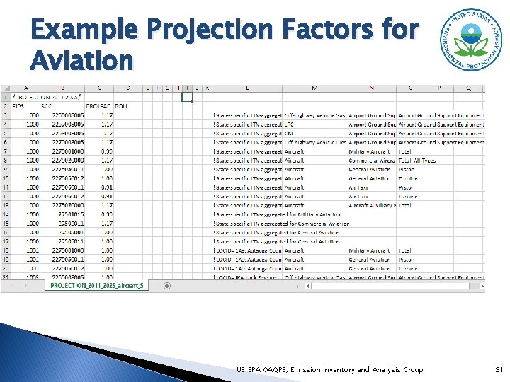
Non-EGU Point Projections: Aviation � Aircraft emissions are in ptnonipm sector � Projected itinerant ITN (i. e. , take off and landing) operations information available from the Federal Aviation Administration’s (FAA) Terminal Area Forecast (TAF) System: � https: //www. faa. gov/data_research/aviation/taf/ � Two sets of projections factors used: ◦ State-level for low traffic airports ◦ Airport specific factors for larger airports US EPA OAQPS, Emission Inventory and Analysis Group 90

Example Projection Factors for Aviation US EPA OAQPS, Emission Inventory and Analysis Group 91

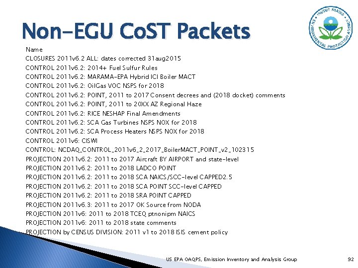
Non-EGU Co. ST Packets Name CLOSURES 2011 v 6. 2 ALL: dates corrected 31 aug 2015 CONTROL 2011 v 6. 2: 2014+ Fuel Sulfur Rules CONTROL 2011 v 6. 2: MARAMA-EPA Hybrid ICI Boiler MACT CONTROL 2011 v 6. 2: Oil. Gas VOC NSPS for 2018 CONTROL 2011 v 6. 2: POINT, 2011 to 2017 Consent decrees and (2018 docket) comments CONTROL 2011 v 6. 2: POINT, 2011 to 20 XX AZ Regional Haze CONTROL 2011 v 6. 2: RICE NESHAP Final Amendments CONTROL 2011 v 6. 2: SCA Gas Turbines NSPS NOX for 2018 CONTROL 2011 v 6. 2: SCA Process Heaters NSPS NOX for 2018 CONTROL 2011 v 6: CISWI CONTROL: NCDAQ_CONTROL_2011 v 6_2_2017_Boiler. MACT_POINT_v 2_102315 PROJECTION 2011 v 6. 2: 2011 to 2017 Aircraft BY AIRPORT and state-level PROJECTION 2011 v 6. 2: 2011 to 2018 LADCO POINT PROJECTION 2011 v 6. 2: 2011 to 2018 SCA NAICS/SCC-level CAPPED 2. 5 PROJECTION 2011 v 6. 2: 2011 to 2018 SCA POINT SCC-level CAPPED PROJECTION 2011 v 6. 2: 2011 to 2018 SRA POINT CAPPED PROJECTION 2011 v 6. 3: 2011 to 2017 OK Source from NODA PROJECTION 2011 v 6: 2011 to 2018 TCEQ ptnonipm NAICS PROJECTION 2011 v 6: 2011 to 2018 state comments PROJECTION by CENSUS DIVISION: 2011 v 1 to 2018 ISIS cement policy US EPA OAQPS, Emission Inventory and Analysis Group 92

Non-EGU Control Packet: ICI Boiler (MACT) � EPA-MJO “hybrid” method: ◦ Council of Industrial Boiler Owners (CIBO) data was collected analyzed to determine how boiler emissions might change due to regulations and economics (i. e. , replacements and conversions) ◦ Impacts nonpoint and specific point sources ◦ Includes NOX cobenefits ◦ Set of fuel-based control assumptions (i. e. , coal, distillate and residual) � Includes NY, NJ some state comments plus rules for US EPA OAQPS, Emission Inventory and Analysis Group 93

Non-EGU Projections: Non-Co. ST � Some future-year sources do not exist in the NEI for the base year ◦ Biodiesel and cellulosic ethanol plants ◦ Other sources added based on comments � Take emissions for these sources as they are reported / provided ◦ These are put into separate inventory files ◦ Hard to project to additional future years US EPA OAQPS, Emission Inventory and Analysis Group 94

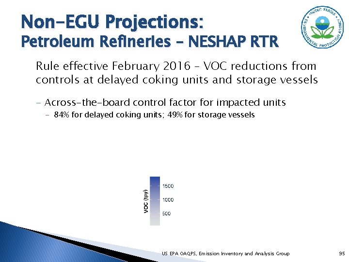
Non-EGU Projections: Petroleum Refineries – NESHAP RTR Rule effective February 2016 – VOC reductions from controls at delayed coking units and storage vessels - Across-the-board control factor for impacted units - 84% for delayed coking units; 49% for storage vessels US EPA OAQPS, Emission Inventory and Analysis Group 95

Non-EGU Projections: CISWI Units – NSPS and Emission Guidelines - Considers the MACT for incinerators, energy recovery units, waste -burning kilns, small, remote incinerators - All impacted units are to have control devices in place by 2018 Existing control devices and baseline emissions based on a 2008 -2009 Information Collection Request Floor emissions represent all units’ emissions after employing least-cost controls to meet MACT standard US EPA OAQPS, Emission Inventory and Analysis Group 96

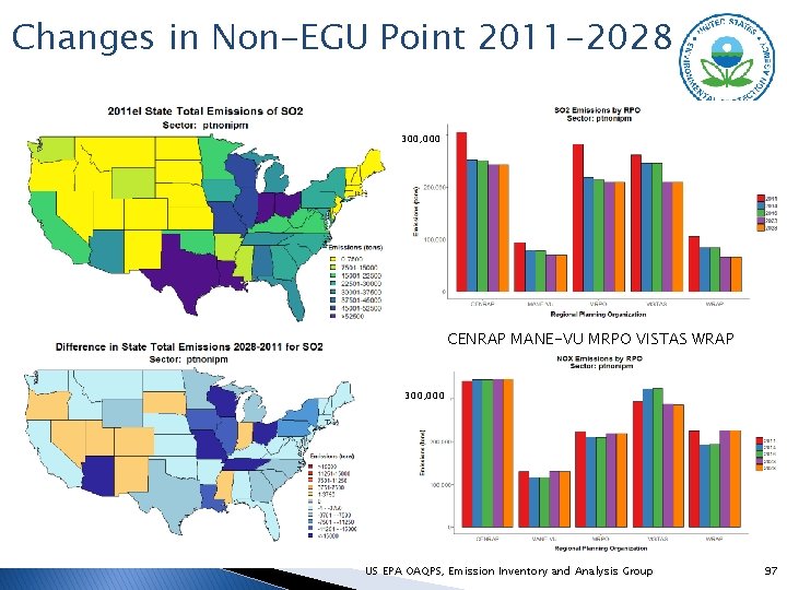
Changes in Non-EGU Point 2011 -2028 300, 000 CENRAP MANE-VU MRPO VISTAS WRAP 300, 000 US EPA OAQPS, Emission Inventory and Analysis Group 97

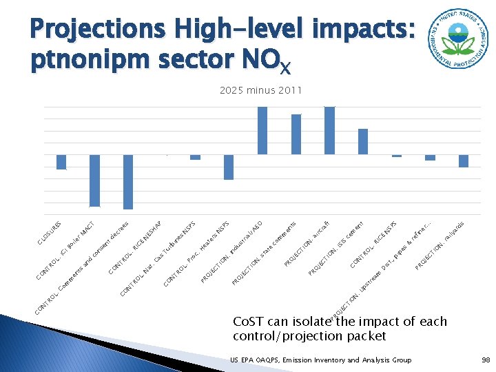
JE O PR tr ps : U N CT IO ea m US EPA OAQPS, Emission Inventory and Analysis Group & ds ar ly ai . . er. fin re SP S N t en ce m CE RI S N : r O CT I pi pe s JE O PR t. , is D L: O N TR CO ra ft irc N : a SI : I N IO CT JE O ts en m m co O AE S N SP SP S N l/ ria st IO CT JE O PR te ta : s N CT IO PR JE nd u N : I rs te . H ea oc es AP H ES es cr e AC T M de N in rb CE RI Tu L: as Pr O TI JE C O O PR PR L: O . G at N N TR CO L: O TR N se nt co n r le ES SU R O CL oi IB IC O TR an d N CO ts L: O N TR CO m en m Co CO L: O N TR CO Projections High-level impacts: ptnonipm sector NOX 2025 minus 2011 Co. ST can isolate the impact of each control/projection packet 98

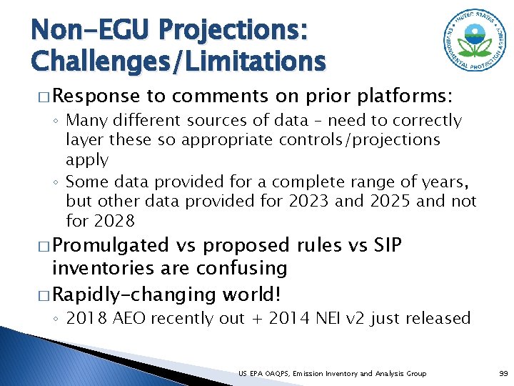
Non-EGU Projections: Challenges/Limitations � Response to comments on prior platforms: ◦ Many different sources of data – need to correctly layer these so appropriate controls/projections apply ◦ Some data provided for a complete range of years, but other data provided for 2023 and 2025 and not for 2028 � Promulgated vs proposed rules vs SIP inventories are confusing � Rapidly-changing world! ◦ 2018 AEO recently out + 2014 NEI v 2 just released US EPA OAQPS, Emission Inventory and Analysis Group 99

Questions on Non-EGU Point? US EPA OAQPS, Emission Inventory and Analysis Group 100

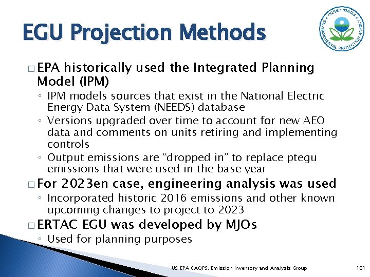
EGU Projection Methods � EPA historically used the Integrated Planning Model (IPM) ◦ IPM models sources that exist in the National Electric Energy Data System (NEEDS) database ◦ Versions upgraded over time to account for new AEO data and comments on units retiring and implementing controls ◦ Output emissions are “dropped in” to replace ptegu emissions that were used in the base year � For 2023 en case, engineering analysis was used ◦ Incorporated historic 2016 emissions and other known upcoming changes to project to 2023 � ERTAC EGU was developed by MJOs ◦ Used for planning purposes US EPA OAQPS, Emission Inventory and Analysis Group 101

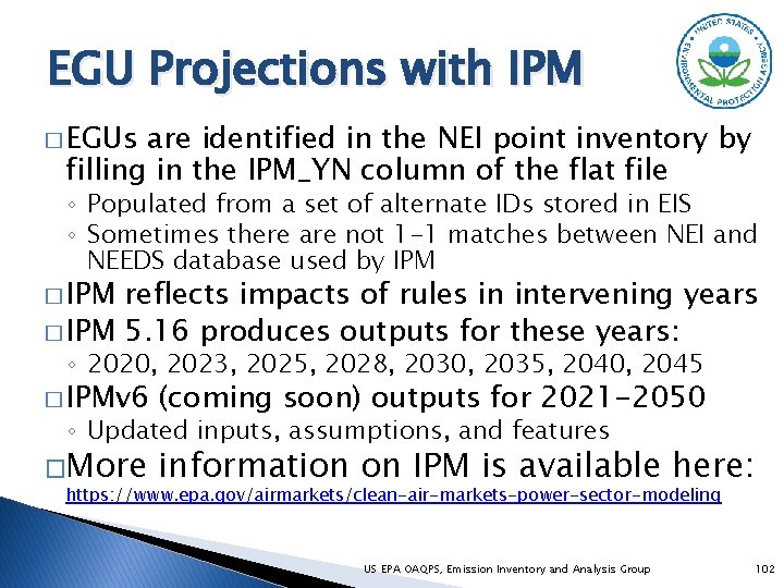
EGU Projections with IPM � EGUs are identified in the NEI point inventory by filling in the IPM_YN column of the flat file ◦ Populated from a set of alternate IDs stored in EIS ◦ Sometimes there are not 1 -1 matches between NEI and NEEDS database used by IPM � IPM reflects impacts of rules in intervening years � IPM 5. 16 produces outputs for these years: ◦ 2020, 2023, 2025, 2028, 2030, 2035, 2040, 2045 � IPMv 6 (coming soon) outputs for 2021 -2050 �More information on IPM is available here: ◦ Updated inputs, assumptions, and features https: //www. epa. gov/airmarkets/clean-air-markets-power-sector-modeling US EPA OAQPS, Emission Inventory and Analysis Group 102

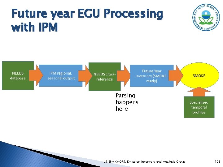
Future year EGU Processing with IPM Parsing happens here US EPA OAQPS, Emission Inventory and Analysis Group 103

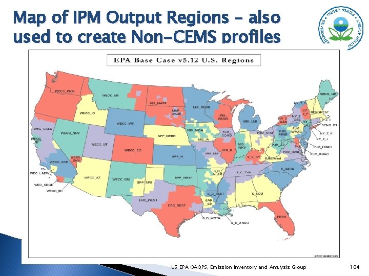
Map of IPM Output Regions – also used to create Non-CEMS profiles US EPA OAQPS, Emission Inventory and Analysis Group 104

Flat Files Created from IPM Outputs � IPM regional, seasonal outputs are converted to a Flat File format that can be input to SMOKE 1. For a specific model output year, parse results to unitlevel for each season (Pollutants = NOx, SO 2, Hg, CO 2) 2. SMOKE-ready Flat file is created from parsed file �Cross reference from National Electric Energy Data System (NEEDS) to NEI units is used to assign NEI-compatible IDs, locations, stack parameters (improved with state review) �PM emissions are created as a postprocess based on emission factors, fuel, and control information � The base year EGU inventory is fully replaced by the flat file inventory output from IPM ◦ IPM results not used in air quality modeling for municipal waste combustors, geothermal, nuclear, wind, solar, or hydro US EPA OAQPS, Emission Inventory and Analysis Group 105

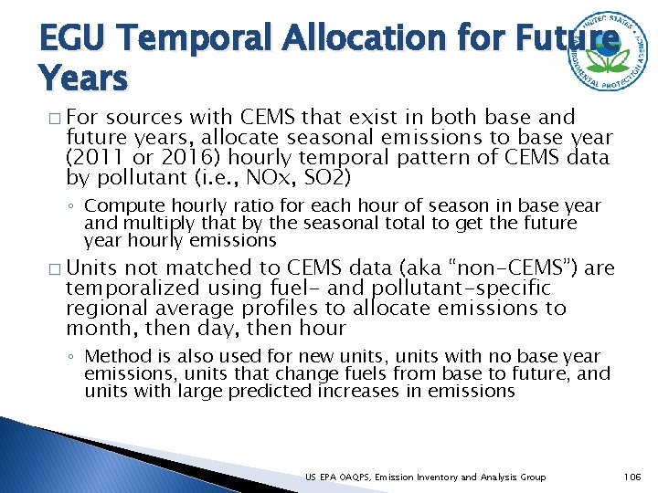
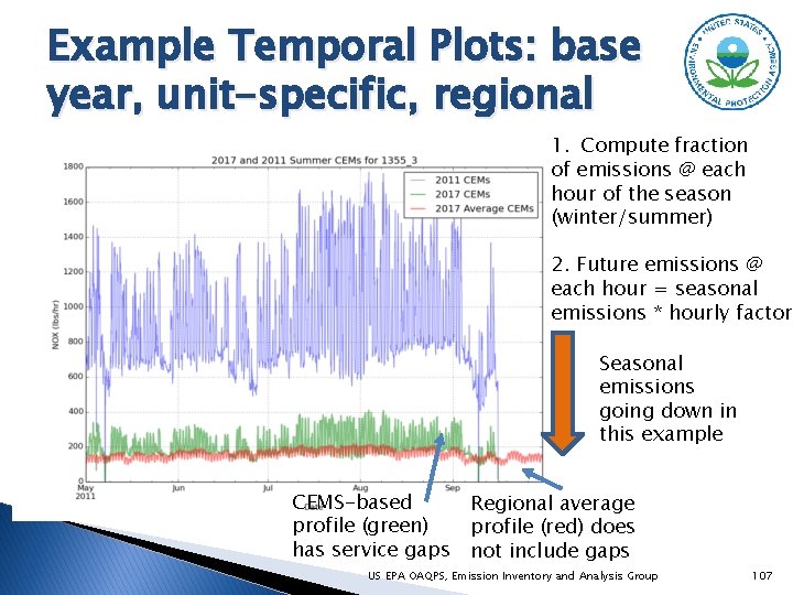
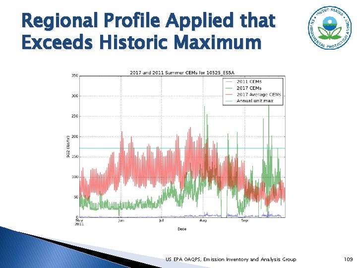
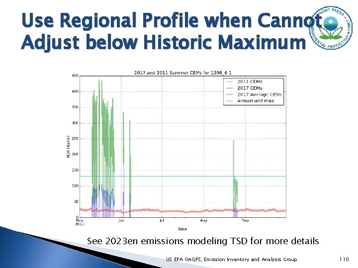
EGU Temporal Allocation for Future Years � For sources with CEMS that exist in both base and future years, allocate seasonal emissions to base year (2011 or 2016) hourly temporal pattern of CEMS data by pollutant (i. e. , NOx, SO 2) ◦ Compute hourly ratio for each hour of season in base year and multiply that by the seasonal total to get the future year hourly emissions � Units not matched to CEMS data (aka “non-CEMS”) are temporalized using fuel- and pollutant-specific regional average profiles to allocate emissions to month, then day, then hour ◦ Method is also used for new units, units with no base year emissions, units that change fuels from base to future, and units with large predicted increases in emissions US EPA OAQPS, Emission Inventory and Analysis Group 106

Example Temporal Plots: base year, unit-specific, regional 1. Compute fraction of emissions @ each hour of the season (winter/summer) 2. Future emissions @ each hour = seasonal emissions * hourly factor Seasonal emissions going down in this example CEMS-based profile (green) has service gaps Regional average profile (red) does not include gaps US EPA OAQPS, Emission Inventory and Analysis Group 107

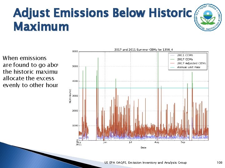
Adjust Emissions Below Historic Maximum When emissions are found to go above the historic maximum, allocate the excess evenly to other hours US EPA OAQPS, Emission Inventory and Analysis Group 108

Regional Profile Applied that Exceeds Historic Maximum US EPA OAQPS, Emission Inventory and Analysis Group 109

Use Regional Profile when Cannot Adjust below Historic Maximum See 2023 en emissions modeling TSD for more details US EPA OAQPS, Emission Inventory and Analysis Group 110

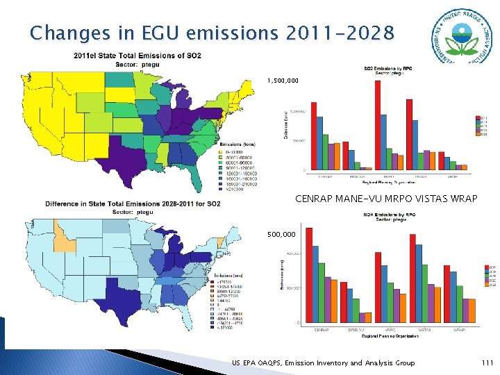
Changes in EGU emissions 2011 -2028 1, 500, 000 CENRAP MANE-VU MRPO VISTAS WRAP 500, 000 US EPA OAQPS, Emission Inventory and Analysis Group 111

Questions? � Any questions on EGU projections? US EPA OAQPS, Emission Inventory and Analysis Group 112

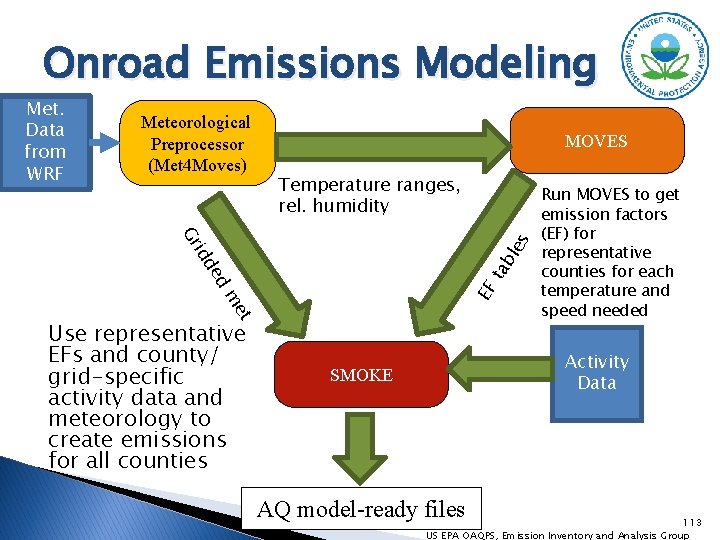
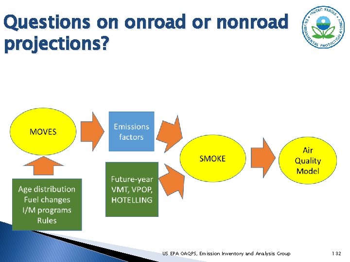
Onroad Emissions Modeling Met. Data from WRF Meteorological Preprocessor (Met 4 Moves) MOVES Temperature ranges, rel. humidity et m EF d ta de bl es id Gr Use representative EFs and county/ grid-specific activity data and meteorology to create emissions for all counties Run MOVES to get emission factors (EF) for representative counties for each temperature and speed needed Activity Data SMOKE AQ model-ready files 113 US EPA OAQPS, Emission Inventory and Analysis Group

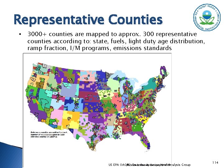
Representative Counties • 3000+ counties are mapped to approx. 300 representative counties according to: state, fuels, light duty age distribution, ramp fraction, I/M programs, emissions standards US EPA OAQPS, Emission Inventory and Analysis Group 114

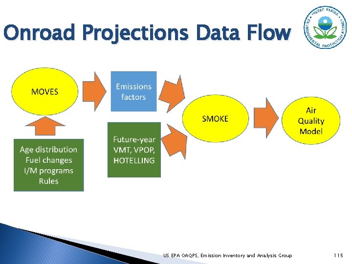
Onroad Projections Data Flow US EPA OAQPS, Emission Inventory and Analysis Group 115

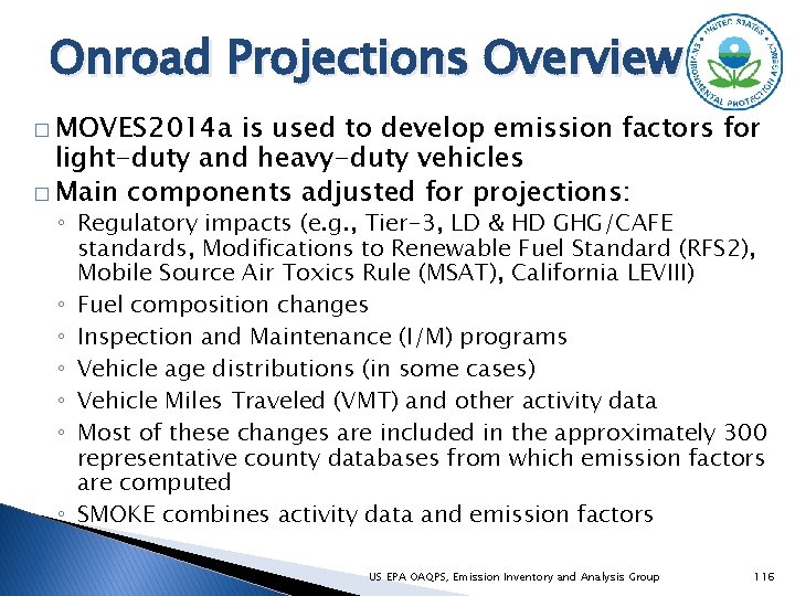
Onroad Projections Overview � MOVES 2014 a is used to develop emission factors for light-duty and heavy-duty vehicles � Main components adjusted for projections: ◦ Regulatory impacts (e. g. , Tier-3, LD & HD GHG/CAFE standards, Modifications to Renewable Fuel Standard (RFS 2), Mobile Source Air Toxics Rule (MSAT), California LEVIII) ◦ Fuel composition changes ◦ Inspection and Maintenance (I/M) programs ◦ Vehicle age distributions (in some cases) ◦ Vehicle Miles Traveled (VMT) and other activity data ◦ Most of these changes are included in the approximately 300 representative county databases from which emission factors are computed ◦ SMOKE combines activity data and emission factors US EPA OAQPS, Emission Inventory and Analysis Group 116

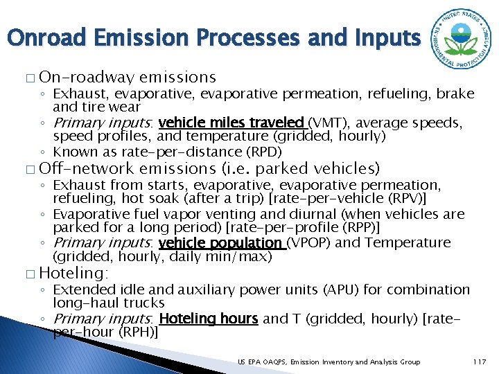
Onroad Emission Processes and Inputs � On-roadway emissions � Off-network emissions (i. e. parked vehicles) ◦ Exhaust, evaporative permeation, refueling, brake and tire wear ◦ Primary inputs: vehicle miles traveled (VMT), average speeds, speed profiles, and temperature (gridded, hourly) ◦ Known as rate-per-distance (RPD) ◦ Exhaust from starts, evaporative permeation, refueling, hot soak (after a trip) [rate-per-vehicle (RPV)] ◦ Evaporative fuel vapor venting and diurnal (when vehicles are parked for a long period) [rate-per-profile (RPP)] ◦ Primary inputs: vehicle population (VPOP) and Temperature (gridded, hourly, daily min/max) � Hoteling: ◦ Extended idle and auxiliary power units (APU) for combination long-haul trucks ◦ Primary inputs: Hoteling hours and T (gridded, hourly) [rateper-hour (RPH)] US EPA OAQPS, Emission Inventory and Analysis Group 117

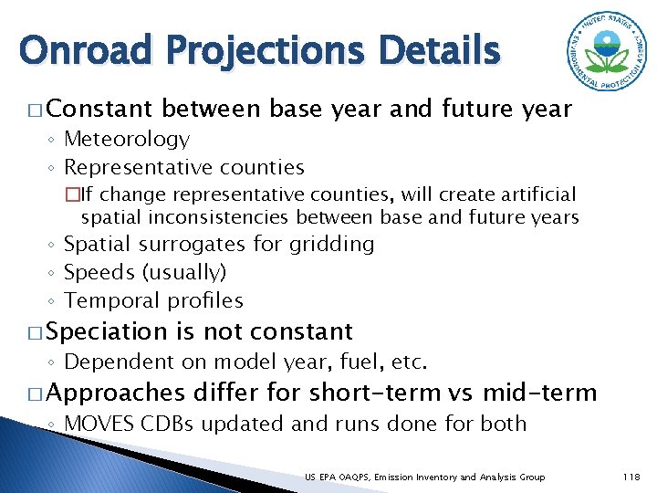
Onroad Projections Details � Constant between base year and future year ◦ Meteorology ◦ Representative counties �If change representative counties, will create artificial spatial inconsistencies between base and future years ◦ Spatial surrogates for gridding ◦ Speeds (usually) ◦ Temporal profiles � Speciation is not constant ◦ Dependent on model year, fuel, etc. � Approaches differ for short-term vs mid-term ◦ MOVES CDBs updated and runs done for both US EPA OAQPS, Emission Inventory and Analysis Group 118

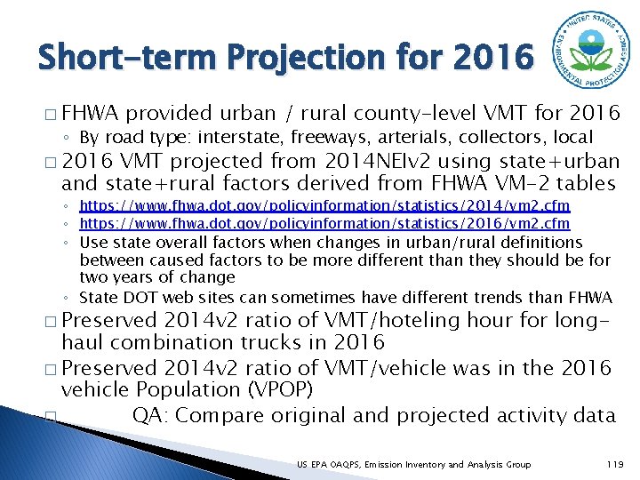
Short-term Projection for 2016 � FHWA provided urban / rural county-level VMT for 2016 ◦ By road type: interstate, freeways, arterials, collectors, local � 2016 VMT projected from 2014 NEIv 2 using state+urban and state+rural factors derived from FHWA VM-2 tables ◦ https: //www. fhwa. dot. gov/policyinformation/statistics/2014/vm 2. cfm ◦ https: //www. fhwa. dot. gov/policyinformation/statistics/2016/vm 2. cfm ◦ Use state overall factors when changes in urban/rural definitions between caused factors to be more different than they should be for two years of change ◦ State DOT web sites can sometimes have different trends than FHWA � Preserved 2014 v 2 ratio of VMT/hoteling hour for longhaul combination trucks in 2016 � Preserved 2014 v 2 ratio of VMT/vehicle was in the 2016 vehicle Population (VPOP) � QA: Compare original and projected activity data US EPA OAQPS, Emission Inventory and Analysis Group 119

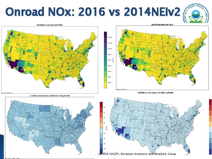
Onroad NOx: 2016 vs 2014 NEIv 2 US EPA OAQPS, Emission Inventory and Analysis Group 120

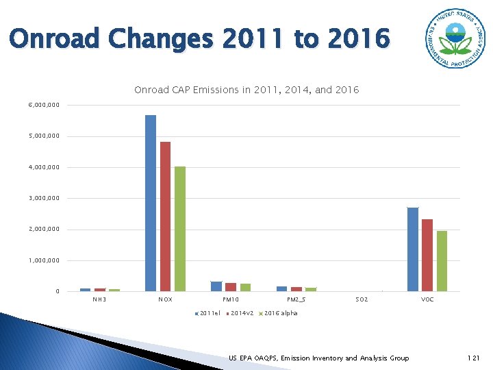
Onroad Changes 2011 to 2016 Onroad CAP Emissions in 2011, 2014, and 2016 6, 000 5, 000 4, 000 3, 000 2, 000 1, 000 0 NH 3 NOX PM 10 2011 el 2014 v 2 PM 2_5 SO 2 VOC 2016 alpha US EPA OAQPS, Emission Inventory and Analysis Group 121

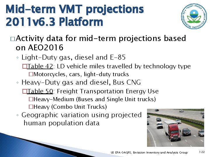
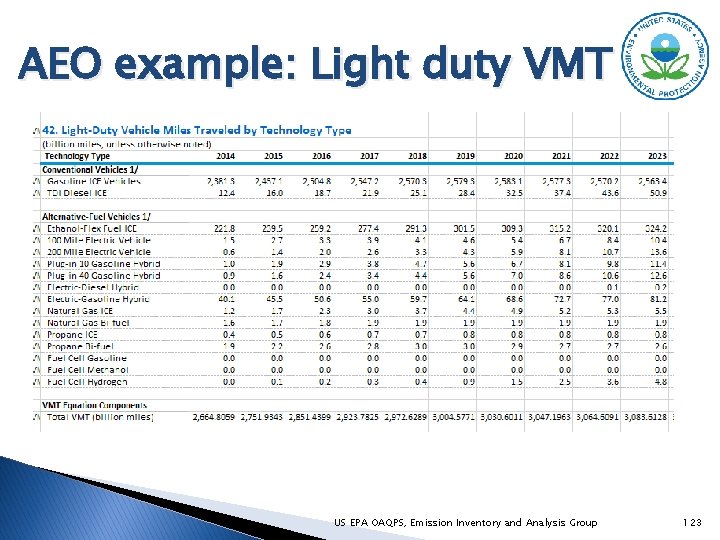
Mid-term VMT projections 2011 v 6. 3 Platform � Activity data for mid-term projections based on AEO 2016 ◦ Light-Duty gas, diesel and E-85 �Table 42: LD vehicle miles travelled by technology type �Motorcycles, cars, light-duty trucks ◦ Heavy-Duty gas and diesel, Bus CNG �Table 50: Freight Transportation Energy Use �Heavy-Medium (Buses and Single Unit trucks) �Heavy (Combo Unit Trucks) ◦ Geographic variation using projected human population data US EPA OAQPS, Emission Inventory and Analysis Group 122

AEO example: Light duty VMT US EPA OAQPS, Emission Inventory and Analysis Group 123

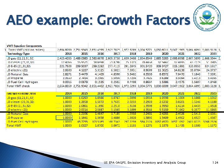
AEO example: Growth Factors US EPA OAQPS, Emission Inventory and Analysis Group 124

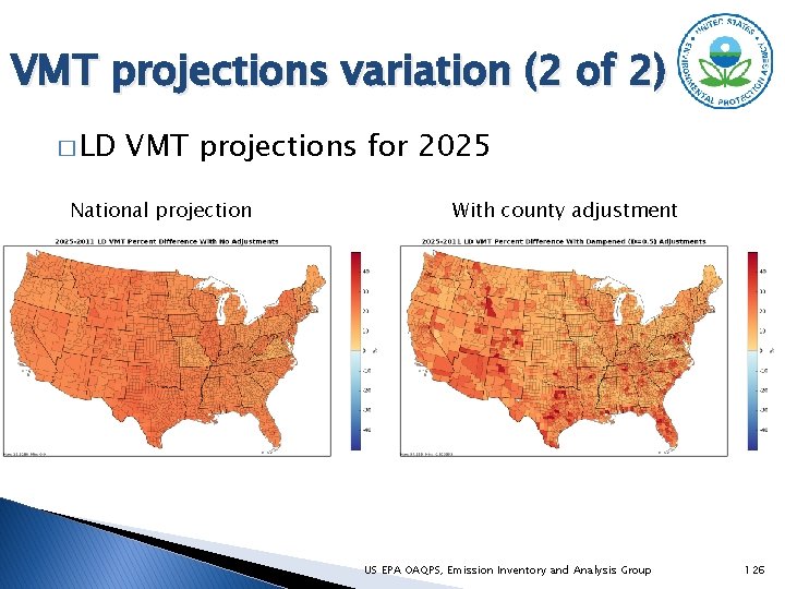
VMT projections variation (1 of 2) � Use AEO 2016 to get magnitude of change � Adjust light duty (LD) VMT projections geographically based on expected human population changes � Analysis indicated strong correlation between population and LD VMT � Correlation between population and medium and heavy duty (MD/HD) VMT is not as strong ◦ Use national factors for medium and heavy duty US EPA OAQPS, Emission Inventory and Analysis Group 125

VMT projections variation (2 of 2) � LD VMT projections for 2025 National projection With county adjustment US EPA OAQPS, Emission Inventory and Analysis Group 126

Onroad Projection Details � Vehicle Population (VPOP) uses same projection factors as VMT � Speciation ◦ Changes in model year and fuels impacts not only the emissions but the speciation ◦ Speciation internal to MOVES 2014 makes it possible to consider detailed model year, regulatory class, and fuel information � Hoteling ◦ Calculate the total hoteling hours from future year combination long-haul restricted VMT ◦ Split between auxiliary power units (APUs) and extended idling (EXT) changes in future years due to greater penetration of APUs US EPA OAQPS, Emission Inventory and Analysis Group 127

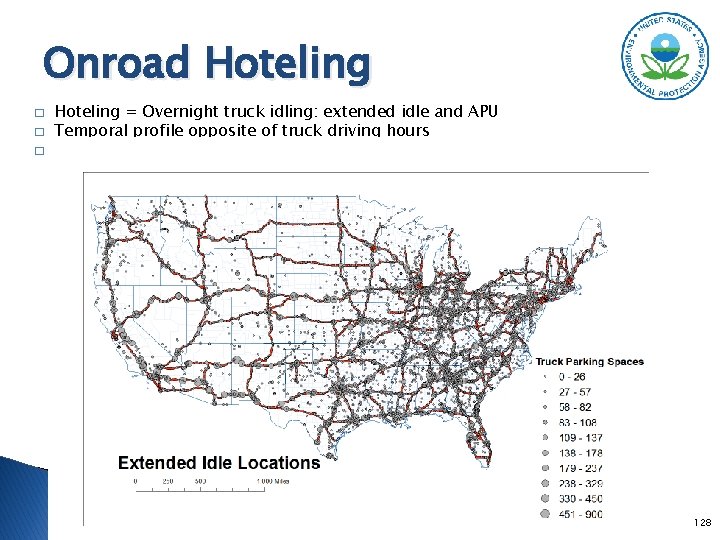
Onroad Hoteling � � � Hoteling = Overnight truck idling: extended idle and APU Temporal profile opposite of truck driving hours Spatial surrogate is based on truck parking spaces 128

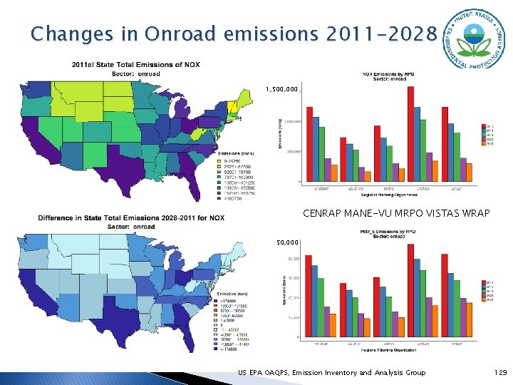
Changes in Onroad emissions 2011 -2028 1, 500, 000 CENRAP MANE-VU MRPO VISTAS WRAP 50, 000 US EPA OAQPS, Emission Inventory and Analysis Group 129

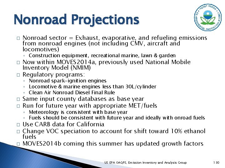
Nonroad Projections � Nonroad sector = Exhaust, evaporative, and refueling emissions from nonroad engines (not including CMV, aircraft and locomotives) ◦ Construction equipment, recreational marine, lawn & garden � � Now within MOVES 2014 a, previously used National Mobile Inventory Model (NMIM) Regulatory programs: ◦ Nonroad spark-ignition engines ◦ Locomotive & marine engines less than 30 L/cylinder ◦ Clean Air Nonroad Diesel Final Rule � � Same input county databases as base year Run for future year with appropriate MET/fuels ◦ Meteorology is consistent with base year ◦ Fuels should be consistent with future year and ideally with onroad fuels � � � Use CARB data for California Change VOC speciation to account for shift toward 10% ethanol fuels MOVES 2014 b coming this summer has updated growth factors US EPA OAQPS, Emission Inventory and Analysis Group 130

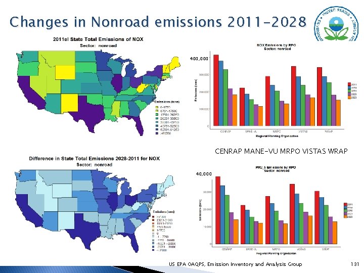
Changes in Nonroad emissions 2011 -2028 400, 000 CENRAP MANE-VU MRPO VISTAS WRAP 40, 000 US EPA OAQPS, Emission Inventory and Analysis Group 131

Questions on onroad or nonroad projections? US EPA OAQPS, Emission Inventory and Analysis Group 132

International Projections � Canada ◦ Base year is 2013 ◦ Projected 2025 Canadian inventory ◦ Interpolate to years in-between � Mexico ◦ Interpolate MOVES-Mexico as needed between 2014, 2017, 2020, 2023 and 2028 ◦ Mexico point, nonroad inventories projected to years 2018, 2025 and 2030 and interpolate as needed US EPA OAQPS, Emission Inventory and Analysis Group 133

Ongoing work and New Directions � 2016 ◦ ◦ ◦ modeling platform Workgroups underway Preparing emissions for 2016, 2023, 2028 Alpha platform for 2016 only currently available Beta platform expected summer-fall V 1. 0 platform expected winter, 2019 � Possible New Directions �Projections of changes in land use/population �Surrogates, New sources, Biogenics, Ag fertilizer �Fires: Impact on biogenics, future year modeling treatment US EPA OAQPS, Emission Inventory and Analysis Group 134

Emissions Modeling Software and Data Downloads � The CMAS Center distributes many tools (https: //www. cmascenter. org/) ◦ SMOKE, CMAQ, VERDI (visualization), the Surrogate Tool, Spatial Allocator, Speciation Tool, and the Control Strategy Tool which includes the Emissions Modeling Framework � SMOKE software and documentation is available from http: //www. cmascenter. org/smoke ◦ A WIKI for SMOKE that answers common questions about emissions modeling is here: https: //www. airqualitymodeling. org/index. php US EPA OAQPS, Emission Inventory and Analysis Group 135

Emissions Modeling Platform Data Availability � EPA’s modeling platform data, documentation, scripts available from ◦ https: //www. epa. gov/air-emissions-modeling ◦ Version 6 platforms include: � 2011 v 6. 3: January 2017 NODA (2011 el/2023 el), Final Cross-State Air Pollution Rule (CSAPR) Update (2011 ek/2017 ek), hemispheric case ◦ ◦ ◦ Version 7. 0 platform for NATA based on 2014 NEIv 1 2016 alpha platform with compatible 2014 and 2015 Spatial surrogates available for 4 km, 12 km, 36 km Speciation data for CB 05, CB 6, SAPRC 07 TB Temporal profiles for all sectors US EPA OAQPS, Emission Inventory and Analysis Group 136

Questions? � Any final questions on the base year part of the training? � Contacts: eyth. alison@epa. gov, Vukovich. jeffrey@epa. gov, farkas. caroline@epa. gov US EPA OAQPS, Emission Inventory and Analysis Group 137