PROJECTILE MOTION Instructions on how to write a

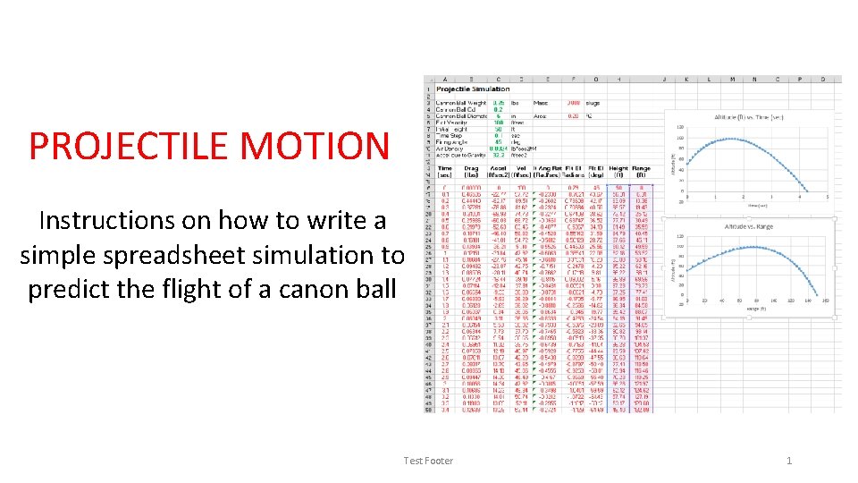
PROJECTILE MOTION Instructions on how to write a simple spreadsheet simulation to predict the flight of a canon ball Test Footer 1

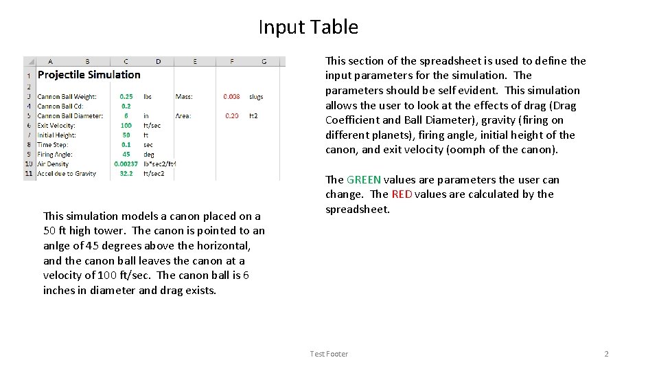
Input Table This section of the spreadsheet is used to define the input parameters for the simulation. The parameters should be self evident. This simulation allows the user to look at the effects of drag (Drag Coefficient and Ball Diameter), gravity (firing on different planets), firing angle, initial height of the canon, and exit velocity (oomph of the canon). This simulation models a canon placed on a 50 ft high tower. The canon is pointed to an anlge of 45 degrees above the horizontal, and the canon ball leaves the canon at a velocity of 100 ft/sec. The canon ball is 6 inches in diameter and drag exists. The GREEN values are parameters the user can change. The RED values are calculated by the spreadsheet. Test Footer 2

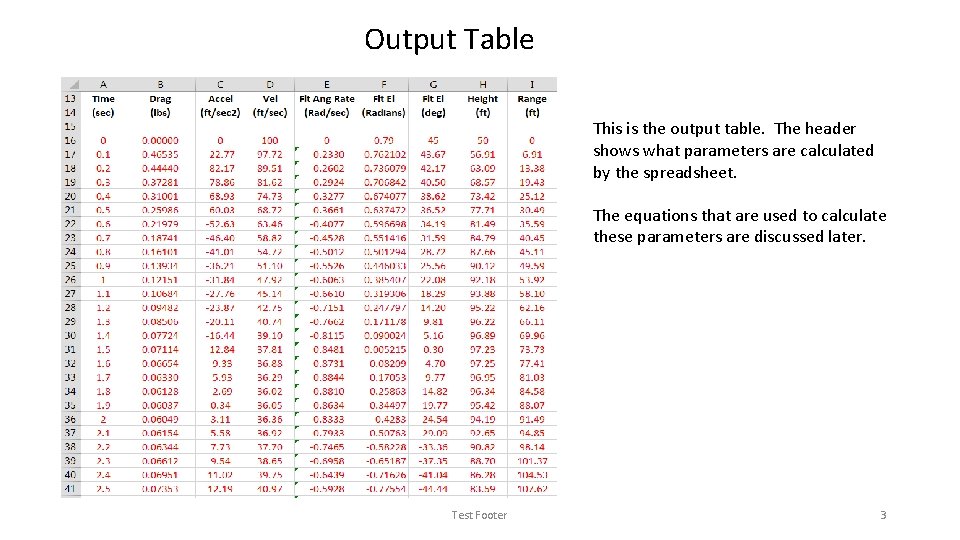
Output Table This is the output table. The header shows what parameters are calculated by the spreadsheet. The equations that are used to calculate these parameters are discussed later. Test Footer 3

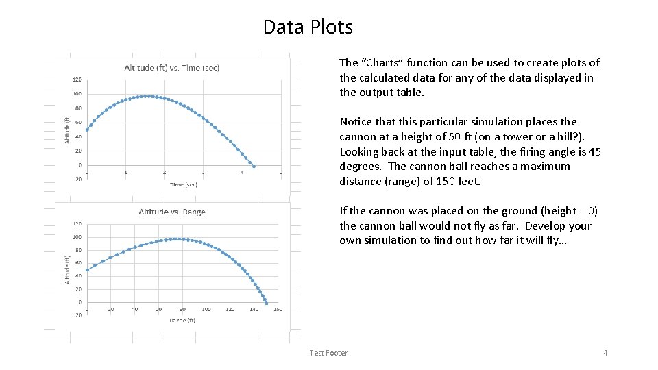
Data Plots The “Charts” function can be used to create plots of the calculated data for any of the data displayed in the output table. Notice that this particular simulation places the cannon at a height of 50 ft (on a tower or a hill? ). Looking back at the input table, the firing angle is 45 degrees. The cannon ball reaches a maximum distance (range) of 150 feet. If the cannon was placed on the ground (height = 0) the cannon ball would not fly as far. Develop your own simulation to find out how far it will fly… Test Footer 4

It is assumed that the student understands the basics of using a spreadsheet, but clarifying descriptions are provide to assist the novice. This simulation performs the “numerical integration” using the Euler method. Refer to the Lab. Rats Lesson on Numerical Integration for a detailed explanation of what is meant by “integration” and how it is accomplished using a computer. The student should also examine the Lab. Rats Projectile Motion Physics Lesson to understand the math and science behind the simulation. This lesson provides the information need to develop a simple simulation of a canon ball being shot out of a canon… Let’s dive into the details… Test Footer 5

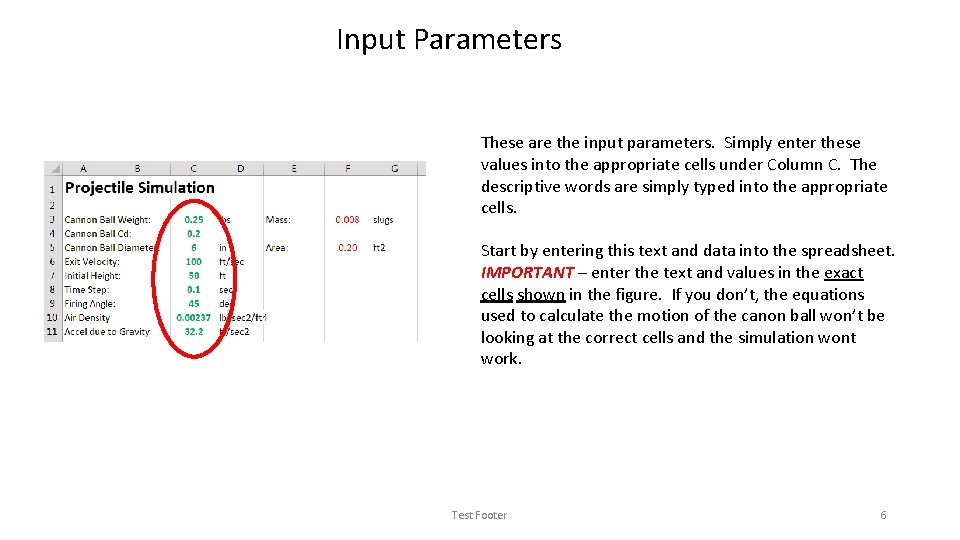
Input Parameters These are the input parameters. Simply enter these values into the appropriate cells under Column C. The descriptive words are simply typed into the appropriate cells. Start by entering this text and data into the spreadsheet. IMPORTANT – enter the text and values in the exact cells shown in the figure. If you don’t, the equations used to calculate the motion of the canon ball won’t be looking at the correct cells and the simulation wont work. Test Footer 6

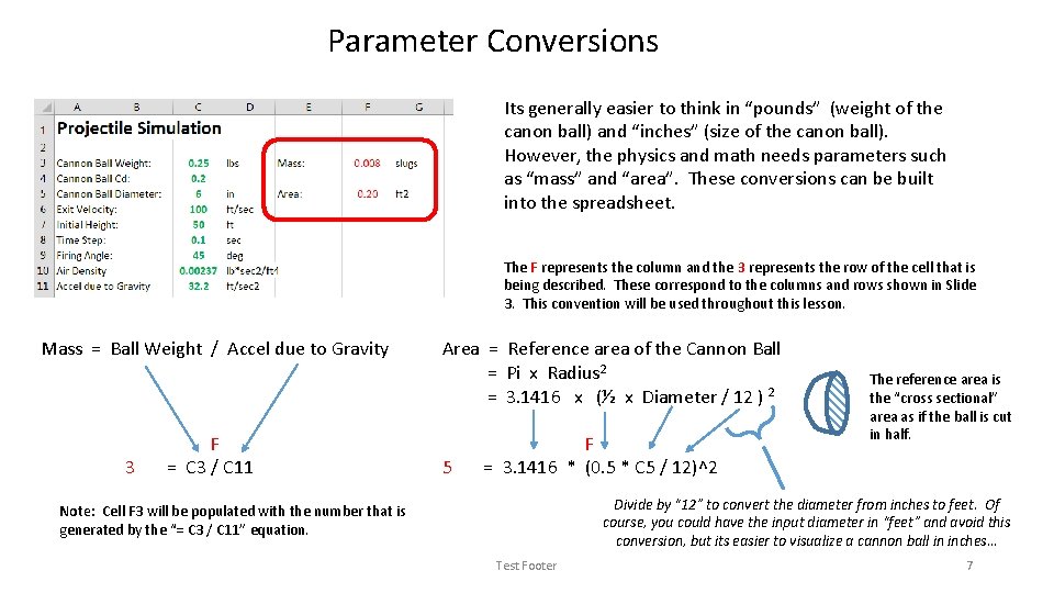
Parameter Conversions Its generally easier to think in “pounds” (weight of the canon ball) and “inches” (size of the canon ball). However, the physics and math needs parameters such as “mass” and “area”. These conversions can be built into the spreadsheet. The F represents the column and the 3 represents the row of the cell that is being described. These correspond to the columns and rows shown in Slide 3. This convention will be used throughout this lesson. Mass = Ball Weight / Accel due to Gravity 3 F = C 3 / C 11 Area = Reference area of the Cannon Ball = Pi x Radius 2 = 3. 1416 x (½ x Diameter / 12 ) 2 5 F = 3. 1416 * (0. 5 * C 5 / 12)^2 The reference area is the “cross sectional” area as if the ball is cut in half. Divide by “ 12” to convert the diameter from inches to feet. Of course, you could have the input diameter in “feet” and avoid this conversion, but its easier to visualize a cannon ball in inches… Note: Cell F 3 will be populated with the number that is generated by the “= C 3 / C 11” equation. Test Footer 7

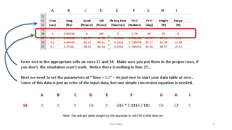
A B C D E F G H I Enter text in the appropriate cells on rows 13 and 14. Make sure you put them in the proper rows, if you don’t, the simulation won’t work. Notice there is nothing in Row 15… Next we need to set the parameters at “Time = 0. 0” – its just nice to start your data table at zero… Some of this data is just an echo of the input data, but one simple conversion equation is needed. 16 A B C D E 0 0 0 C 6 0 F G 16 * 3. 1416 / 180 G H I C 9 C 7 0 Note: You will get some insight on the equation in cell F 16 a little later on Test Footer 8

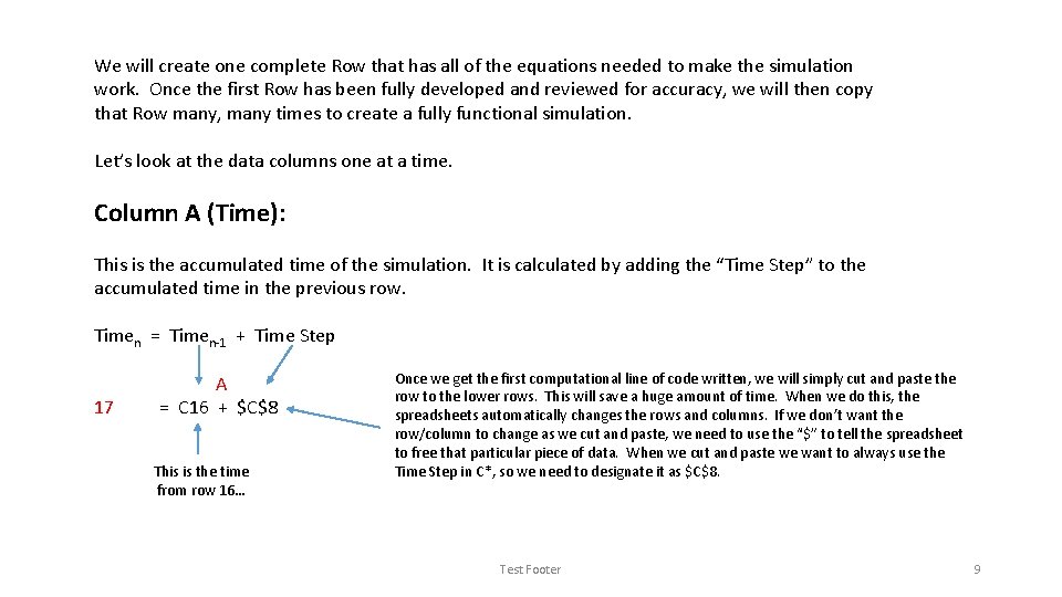
We will create one complete Row that has all of the equations needed to make the simulation work. Once the first Row has been fully developed and reviewed for accuracy, we will then copy that Row many, many times to create a fully functional simulation. Let’s look at the data columns one at a time. Column A (Time): This is the accumulated time of the simulation. It is calculated by adding the “Time Step” to the accumulated time in the previous row. Timen = Timen-1 + Time Step 17 A = C 16 + $C$8 This is the time from row 16… Once we get the first computational line of code written, we will simply cut and paste the row to the lower rows. This will save a huge amount of time. When we do this, the spreadsheets automatically changes the rows and columns. If we don’t want the row/column to change as we cut and paste, we need to use the “$” to tell the spreadsheet to free that particular piece of data. When we cut and paste we want to always use the Time Step in C*, so we need to designate it as $C$8. Test Footer 9

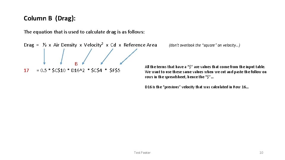
Column B (Drag): The equation that is used to calculate drag is as follows: Drag = ½ x Air Density x Velocity 2 x Cd x Reference Area 17 B = 0. 5 * $C$10 * D 16^2 * $C$4 * $F$5 (don’t overlook the “square” on velocity…) All the terms that have a “$” are values that come from the input table. We want to use these same values when we cut and paste the follow on rows in the spreadsheet, hence the “$”… D 16 is the “previous” velocity that was calculated in Row 16… Test Footer 10

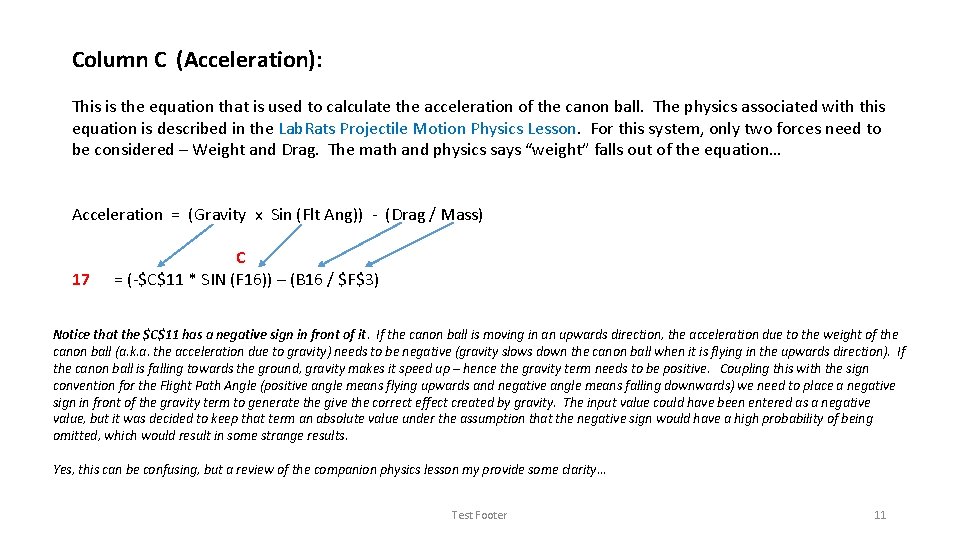
Column C (Acceleration): This is the equation that is used to calculate the acceleration of the canon ball. The physics associated with this equation is described in the Lab. Rats Projectile Motion Physics Lesson. For this system, only two forces need to be considered – Weight and Drag. The math and physics says “weight” falls out of the equation… Acceleration = (Gravity x Sin (Flt Ang)) - (Drag / Mass) 17 C = (-$C$11 * SIN (F 16)) – (B 16 / $F$3) Notice that the $C$11 has a negative sign in front of it. If the canon ball is moving in an upwards direction, the acceleration due to the weight of the canon ball (a. k. a. the acceleration due to gravity) needs to be negative (gravity slows down the canon ball when it is flying in the upwards direction). If the canon ball is falling towards the ground, gravity makes it speed up – hence the gravity term needs to be positive. Coupling this with the sign convention for the Flight Path Angle (positive angle means flying upwards and negative angle means falling downwards) we need to place a negative sign in front of the gravity term to generate the give the correct effect created by gravity. The input value could have been entered as a negative value, but it was decided to keep that term an absolute value under the assumption that the negative sign would have a high probability of being omitted, which would result in some strange results. Yes, this can be confusing, but a review of the companion physics lesson my provide some clarity… Test Footer 11

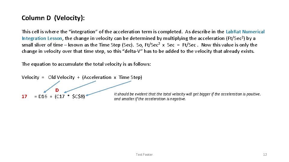
Column D (Velocity): This cell is where the “integration” of the acceleration term is completed. As describe in the Lab. Rat Numerical Integration Lesson, the change in velocity can be determined by multiplying the acceleration (Ft/Sec 2) by a small sliver of time – known as the Time Step (Sec). So, Ft/Sec 2 x Sec = Ft/Sec. Now this value is only the change in velocity over that time step, so this “delta-V” has to be added to the velocity that already exists. The equation to accumulate the total velocity is as follows: Velocity = Old Velocity + (Acceleration x Time Step) 17 D = D 16 + (C 17 * $C$8) It should be evident that the total velocity will get bigger if the acceleration is positive, and smaller if the acceleration is negative. Test Footer 12

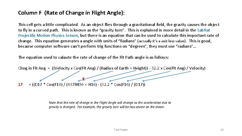
Column F (Rate of Change in Flight Angle): This cell gets a little complicated. As an object flies through a gravitational field, the gravity causes the object to fly in a curved path. This is known as the “gravity turn”. This is explained in more detail in the Lab. Rat Projectile Motion Physics Lesson, but there is an equation that can be used to calculate this important rate of change. This equation generates a angle with units of “Radians” (actually it’s a unit less value). This is good, because computer software can’t perform trig functions on “degrees”, they must use “radians”… The equation used to calaute the rate of change of the Flt Path angle is as follows: Chng in Flt Ang = ((Velocity x Cos(Flt Ang) / (Radius of Earth + Height)) - 32. 2 x Cos(Flt Ang) / Velocity) 17 E = ((D 17 * Cos(F 16) / (6378456 + H 16) - (32. 2 * Cos(F 16) / (D 17)) Note that the rate of change in the Flight Angle will change as the acceleration due to gravity is changed. For example, the gravity turn will be less severe on the moon. Test Footer 13

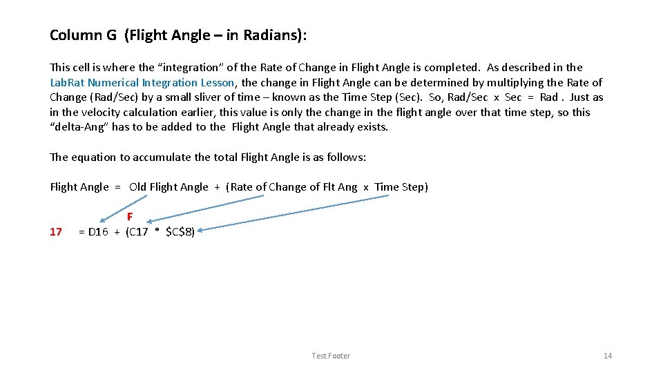
Column G (Flight Angle – in Radians): This cell is where the “integration” of the Rate of Change in Flight Angle is completed. As described in the Lab. Rat Numerical Integration Lesson, the change in Flight Angle can be determined by multiplying the Rate of Change (Rad/Sec) by a small sliver of time – known as the Time Step (Sec). So, Rad/Sec x Sec = Rad. Just as in the velocity calculation earlier, this value is only the change in the flight angle over that time step, so this “delta-Ang” has to be added to the Flight Angle that already exists. The equation to accumulate the total Flight Angle is as follows: Flight Angle = Old Flight Angle + (Rate of Change of Flt Ang x Time Step) 17 F = D 16 + (C 17 * $C$8) Test Footer 14

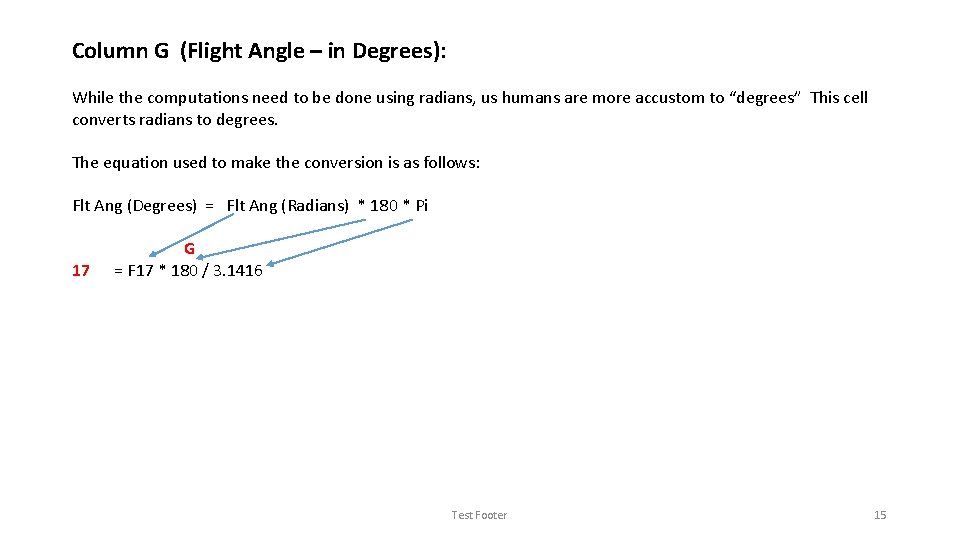
Column G (Flight Angle – in Degrees): While the computations need to be done using radians, us humans are more accustom to “degrees” This cell converts radians to degrees. The equation used to make the conversion is as follows: Flt Ang (Degrees) = Flt Ang (Radians) * 180 * Pi 17 G = F 17 * 180 / 3. 1416 Test Footer 15

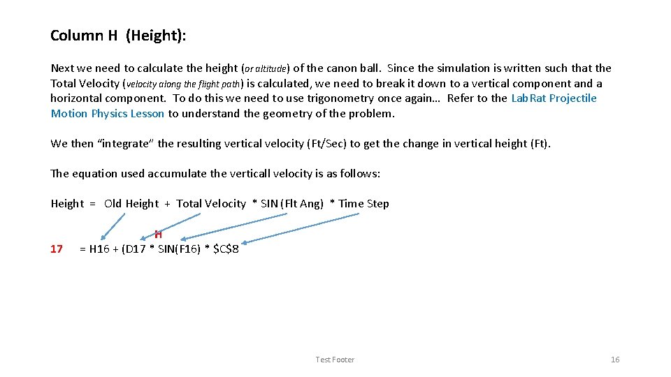
Column H (Height): Next we need to calculate the height (or altitude) of the canon ball. Since the simulation is written such that the Total Velocity (velocity along the flight path) is calculated, we need to break it down to a vertical component and a horizontal component. To do this we need to use trigonometry once again… Refer to the Lab. Rat Projectile Motion Physics Lesson to understand the geometry of the problem. We then “integrate” the resulting vertical velocity (Ft/Sec) to get the change in vertical height (Ft). The equation used accumulate the verticall velocity is as follows: Height = Old Height + Total Velocity * SIN (Flt Ang) * Time Step 17 H = H 16 + (D 17 * SIN(F 16) * $C$8 Test Footer 16

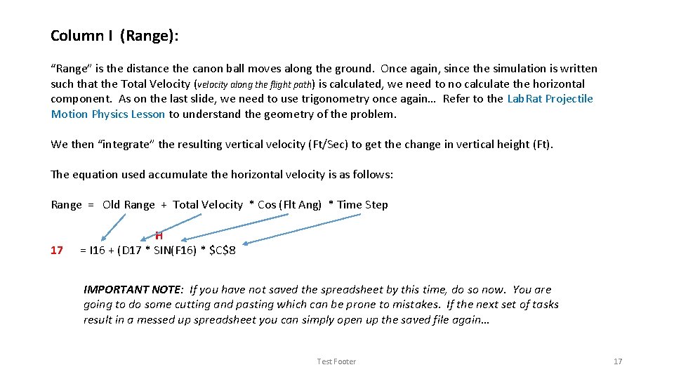
Column I (Range): “Range” is the distance the canon ball moves along the ground. Once again, since the simulation is written such that the Total Velocity (velocity along the flight path) is calculated, we need to no calculate the horizontal component. As on the last slide, we need to use trigonometry once again… Refer to the Lab. Rat Projectile Motion Physics Lesson to understand the geometry of the problem. We then “integrate” the resulting vertical velocity (Ft/Sec) to get the change in vertical height (Ft). The equation used accumulate the horizontal velocity is as follows: Range = Old Range + Total Velocity * Cos (Flt Ang) * Time Step 17 H = I 16 + (D 17 * SIN(F 16) * $C$8 IMPORTANT NOTE: If you have not saved the spreadsheet by this time, do so now. You are going to do some cutting and pasting which can be prone to mistakes. If the next set of tasks result in a messed up spreadsheet you can simply open up the saved file again… Test Footer 17

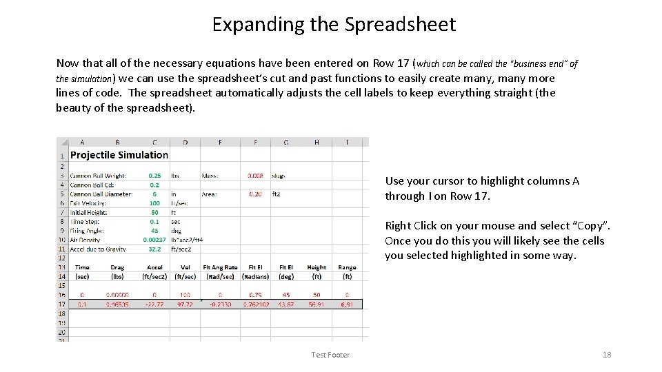
Expanding the Spreadsheet Now that all of the necessary equations have been entered on Row 17 (which can be called the “business end” of the simulation) we can use the spreadsheet’s cut and past functions to easily create many, many more lines of code. The spreadsheet automatically adjusts the cell labels to keep everything straight (the beauty of the spreadsheet). Use your cursor to highlight columns A through I on Row 17. Right Click on your mouse and select “Copy”. Once you do this you will likely see the cells you selected highlighted in some way. Test Footer 18

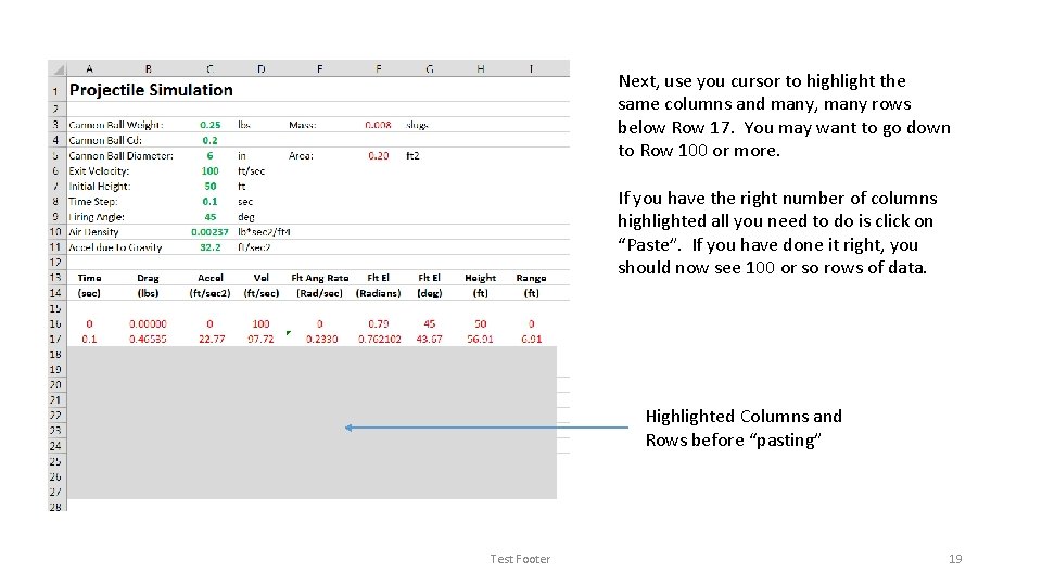
Next, use you cursor to highlight the same columns and many, many rows below Row 17. You may want to go down to Row 100 or more. If you have the right number of columns highlighted all you need to do is click on “Paste”. If you have done it right, you should now see 100 or so rows of data. Highlighted Columns and Rows before “pasting” Test Footer 19

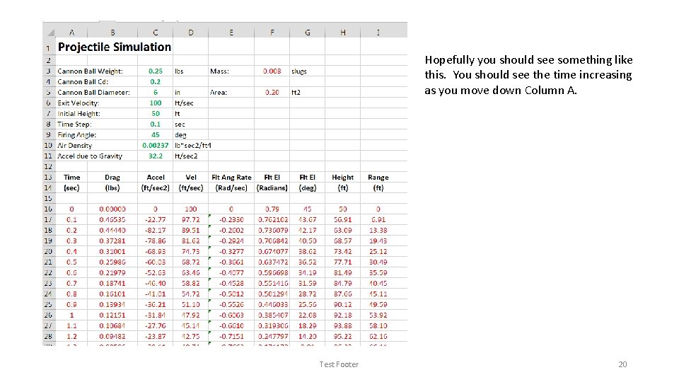
Hopefully you should see something like this. You should see the time increasing as you move down Column A. Test Footer 20

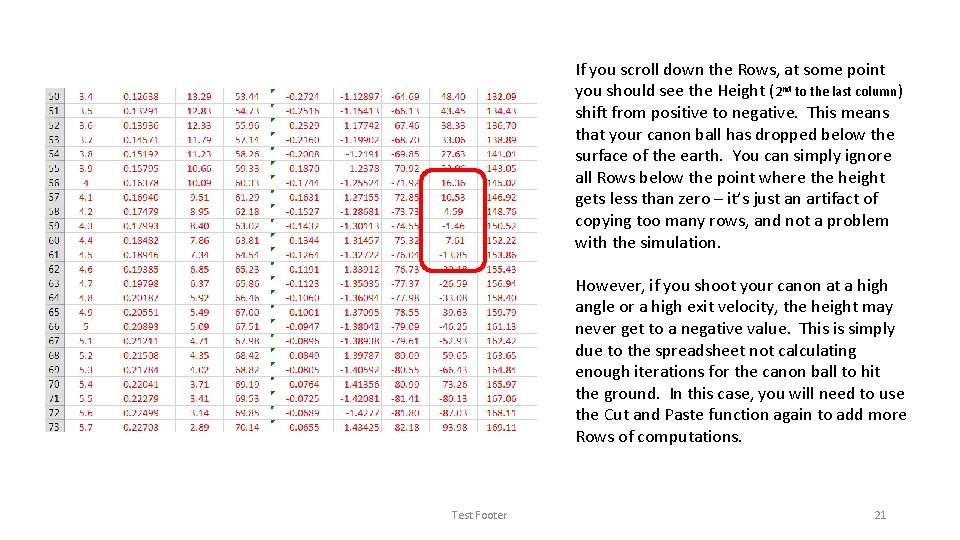
If you scroll down the Rows, at some point you should see the Height (2 nd to the last column) shift from positive to negative. This means that your canon ball has dropped below the surface of the earth. You can simply ignore all Rows below the point where the height gets less than zero – it’s just an artifact of copying too many rows, and not a problem with the simulation. However, if you shoot your canon at a high angle or a high exit velocity, the height may never get to a negative value. This is simply due to the spreadsheet not calculating enough iterations for the canon ball to hit the ground. In this case, you will need to use the Cut and Paste function again to add more Rows of computations. Test Footer 21

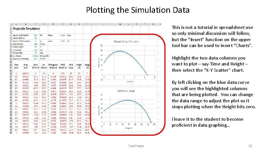
Plotting the Simulation Data This is not a tutorial in spreadsheet use so only minimal discussion will follow, but the “Insert” function on the upper tool bar can be used to insert “Charts”. Highlight the two data columns you want to plot – say Time and Height – then select the “X-Y Scatter” chart. By left clicking on the blue data curve you will see the highlighted columns that are being plotted. You can change the data range to adjust the plot so it stops plotting when the Height hits zero. I leave it to the student to become proficient in data graphing… Test Footer 22

If you get some weird data and some funky data curves you probably have an error in your equations somewhere. Carefully examine each cell in Row 17 to see where the problem is. Once the error is found, simple copy and paste the new Row 17 over the Rows below Row 17. Test Footer 23