Project Initiation Selection and Planning Importance of Project

Project Initiation, Selection, and Planning

Importance of Project Selection “There are two ways for a business to succeed at new projects: doing projects right, and doing the right projects. ” R. G. Cooper, S. Edgett, E. Kleinschmidt. 2000. Research and Technology Management. Good project selection makes the later job of running projects much easier. Also, poorly selected projects may be doomed from the start. On average, companies are less good at project selection than they are at project operation. 2

Different Approaches to Project Selection There are two fundamentally different approaches to project selection. In the first approach, projects are evaluated individually, and that information is used to make a go / no go decision. In the second approach, project selection is viewed as a portfolio planning problem, and the go /no go decisions for all projects are made simultaneously. The second approach, where possible, is much better, since it controls risk through diversification, utilizes resources more efficiently, and optimizes overall performance. 3 Some hybrid approaches may also be useful.

Individual Project Selection Overview 1. Strategic factors Competitive necessity: keep a foothold in the market, not get left behind Market expansion opportunities: not yet profitable, but need to establish a presence Consistency: in line with overall organization’s mission statement Image: potential impact of project on corporate image 4

Individual Project Selection - Overview 2. Project portfolio factors Diversification: reduce market and other risks by maintaining a mix of projects Cash flow constraints: balance available cash over time and across projects Resource constraints: plan available resources (facility, personnel) over time 5

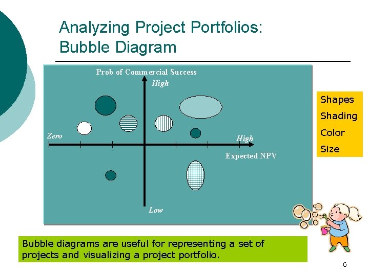
Analyzing Project Portfolios: Bubble Diagram Prob of Commercial Success High Shapes Shading Zero High Expected NPV Color Size Low Bubble diagrams are useful for representing a set of projects and visualizing a project portfolio. 6

Individual Project Selection - Overview 3. Project risk factors Probability of research being successful Probability of development being successful Probability of project success w. r. t. scope Probability of commercial success Overall risk of project Competitors in market and their reactions 7

Individual Project Selection Overview 4. Quantitative factors Payback period Net present value / internal rate of return Expected commercial value Real options Multifactor scoring 8

Payback Period Analysis Number of years needed for the project to repay its initial fixed investment. Example: A project costs $100, 000 and is expected to save the company $20, 000 per year Payback Period = $100, 000 / $20, 000 = 5 years 9

Comments on Payback Period Easy to calculate and explain, and sometimes can be used to achieve a common purpose throughout an organization. ¡ Ignores the time value of money, including interest rates and inflation. ¡ Ignores money earned after the payback period. ¡ 10

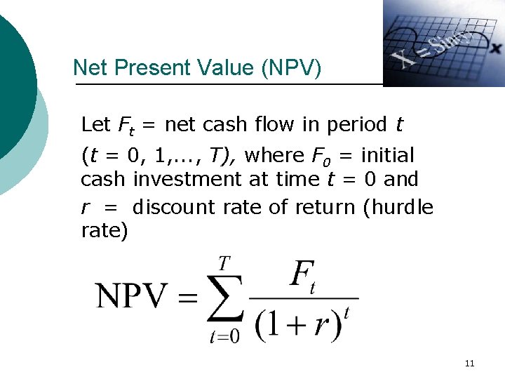
Net Present Value (NPV) Let Ft = net cash flow in period t (t = 0, 1, . . . , T), where F 0 = initial cash investment at time t = 0 and r = discount rate of return (hurdle rate) 11

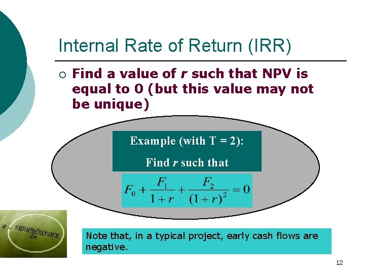
Internal Rate of Return (IRR) ¡ Find a value of r such that NPV is equal to 0 (but this value may not be unique) Example (with T = 2): Find r such that Note that, in a typical project, early cash flows are negative. 12

NPV Example Phase I Research and Product Development: $18 million annual research cost for 2 years. ¡ Phase II Market Development: $10 million annual expenditure for 2 years to develop marketing and distribution channels. ¡ Phase III Sales: All cash flows are after-tax and occur at year's end. ¡ 13

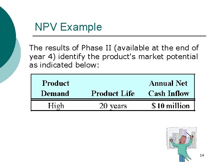
NPV Example The results of Phase II (available at the end of year 4) identify the product's market potential as indicated below: 14

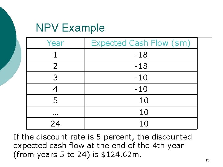
NPV Example Year 1 2 3 4 5 … 24 Expected Cash Flow ($m) -18 -10 10 If the discount rate is 5 percent, the discounted expected cash flow at the end of the 4 th year (from years 5 to 24) is $124. 62 m. 15

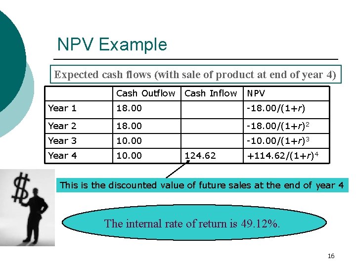
NPV Example Expected cash flows (with sale of product at end of year 4) Cash Outflow Cash Inflow NPV Year 1 18. 00 -18. 00/(1+r) Year 2 18. 00 -18. 00/(1+r)2 Year 3 10. 00 -10. 00/(1+r)3 Year 4 10. 00 124. 62 +114. 62/(1+r)4 This is the discounted value of future sales at the end of year 4 The internal rate of return is 49. 12%. 16

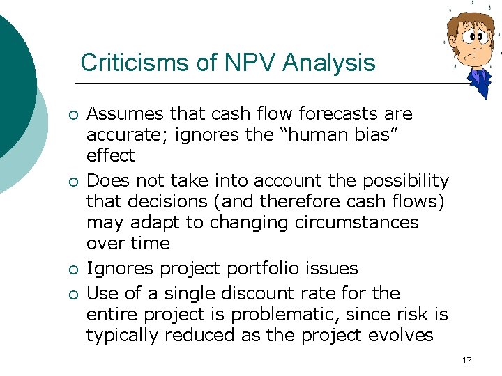
Criticisms of NPV Analysis ¡ ¡ Assumes that cash flow forecasts are accurate; ignores the “human bias” effect Does not take into account the possibility that decisions (and therefore cash flows) may adapt to changing circumstances over time Ignores project portfolio issues Use of a single discount rate for the entire project is problematic, since risk is typically reduced as the project evolves 17

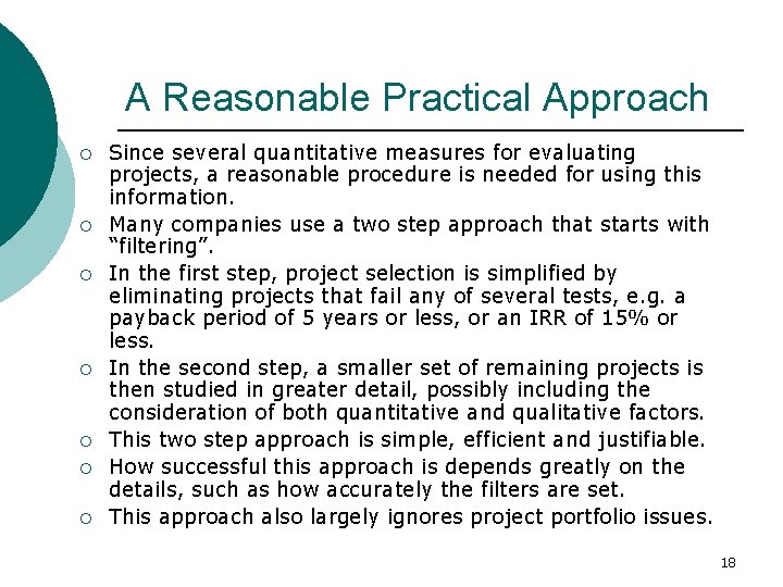
A Reasonable Practical Approach ¡ ¡ ¡ ¡ Since several quantitative measures for evaluating projects, a reasonable procedure is needed for using this information. Many companies use a two step approach that starts with “filtering”. In the first step, project selection is simplified by eliminating projects that fail any of several tests, e. g. a payback period of 5 years or less, or an IRR of 15% or less. In the second step, a smaller set of remaining projects is then studied in greater detail, possibly including the consideration of both quantitative and qualitative factors. This two step approach is simple, efficient and justifiable. How successful this approach is depends greatly on the details, such as how accurately the filters are set. This approach also largely ignores project portfolio issues. 18

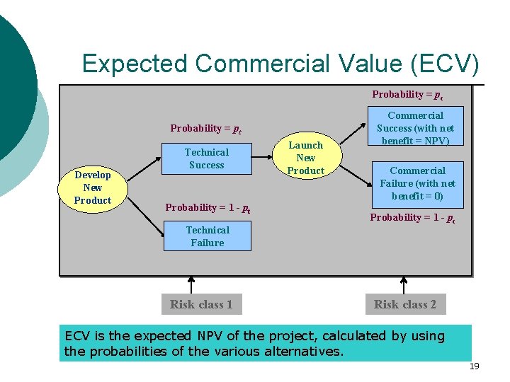
Expected Commercial Value (ECV) Probability = pc Probability = pt Develop New Product Technical Success Probability = 1 - pt Technical Failure Risk class 1 Launch New Product Commercial Success (with net benefit = NPV) Commercial Failure (with net benefit = 0) Probability = 1 - pc Risk class 2 ECV is the expected NPV of the project, calculated by using the probabilities of the various alternatives. 19

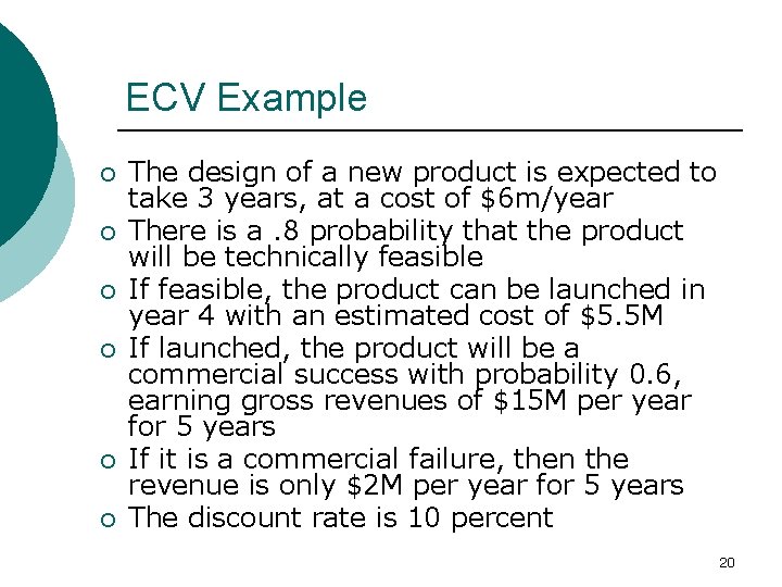
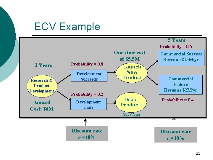
ECV Example ¡ ¡ ¡ The design of a new product is expected to take 3 years, at a cost of $6 m/year There is a. 8 probability that the product will be technically feasible If feasible, the product can be launched in year 4 with an estimated cost of $5. 5 M If launched, the product will be a commercial success with probability 0. 6, earning gross revenues of $15 M per year for 5 years If it is a commercial failure, then the revenue is only $2 M per year for 5 years The discount rate is 10 percent 20

ECV Example 5 Years Probability = 0. 6 3 Years Research & Product Development Annual Cost: $6 M Probability = 0. 8 Development Succeeds One-time cost of $5. 5 M Launch New Product Probability = 0. 2 Development Fails Drop Product Commercial Success Revenue $15 M/yr Commercial Failure Revenue $2 M/yr Probability = 0. 4 No Cost Discount rate r 1=10% Discount rate r 2=10% 21

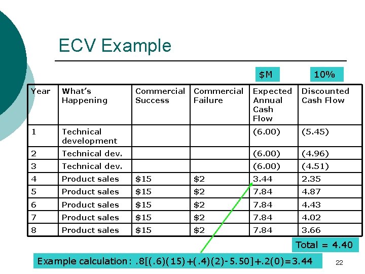
ECV Example $M Year What’s Happening 1 Commercial Success Commercial Failure 10% Expected Annual Cash Flow Discounted Cash Flow Technical development (6. 00) (5. 45) 2 Technical dev. (6. 00) (4. 96) 3 Technical dev. (6. 00) (4. 51) 4 Product sales $15 $2 3. 44 2. 35 5 Product sales $15 $2 7. 84 4. 87 6 Product sales $15 $2 7. 84 4. 43 7 Product sales $15 $2 7. 84 4. 02 8 Product sales $15 $2 7. 84 3. 66 Total = 4. 40 Example calculation: . 8[(. 6)(15)+(. 4)(2)-5. 50]+. 2(0)=3. 44 22

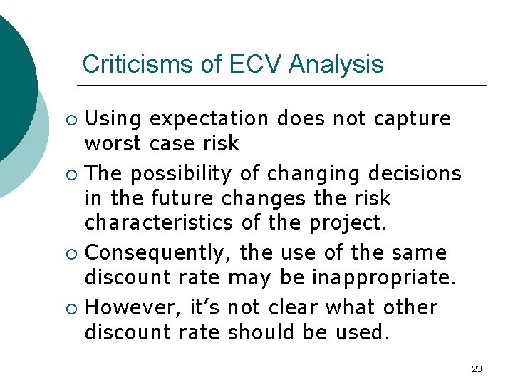
Criticisms of ECV Analysis Using expectation does not capture worst case risk ¡ The possibility of changing decisions in the future changes the risk characteristics of the project. ¡ Consequently, the use of the same discount rate may be inappropriate. ¡ However, it’s not clear what other discount rate should be used. ¡ 23

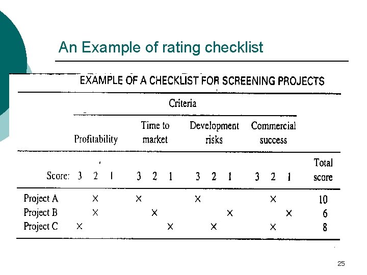
Project Selection The Rating Checklist Approach § Checklist construction § § Identify the criteria or the set of requirements Score each project according to how well it does with respect to each criterion. § § Words such as “excellent”, “good”, “poor”, etc. , are usually assigned with numerical values. Garrison Keillor, “A Prairie Home Companion”: “Lake Wobegon, where all the women are strong, all the men good-looking and all the children are above average”. 24

An Example of rating checklist 25

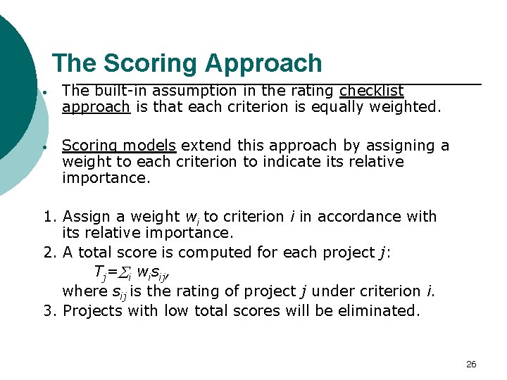
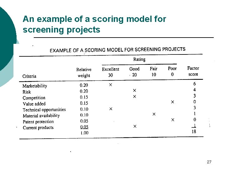
The Scoring Approach · The built-in assumption in the rating checklist approach is that each criterion is equally weighted. · Scoring models extend this approach by assigning a weight to each criterion to indicate its relative importance. 1. Assign a weight wi to criterion i in accordance with its relative importance. 2. A total score is computed for each project j: Tj= i wisij, where sij is the rating of project j under criterion i. 3. Projects with low total scores will be eliminated. 26

An example of a scoring model for screening projects 27

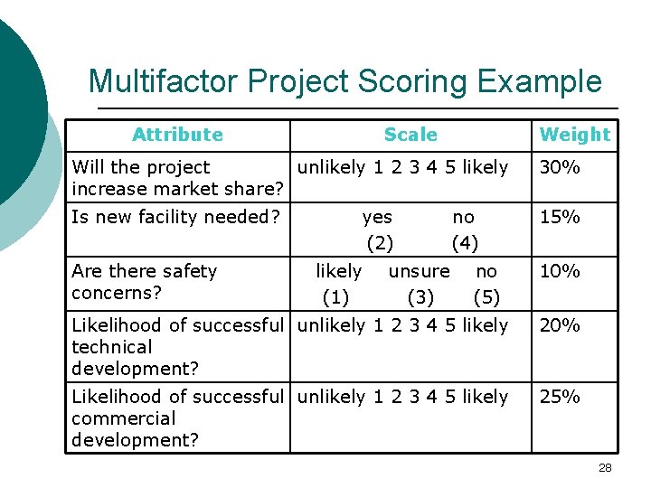
Multifactor Project Scoring Example Attribute Scale Weight Will the project unlikely 1 2 3 4 5 likely increase market share? 30% Is new facility needed? 15% Are there safety concerns? yes (2) likely (1) unsure (3) no (4) no (5) 10% Likelihood of successful unlikely 1 2 3 4 5 likely technical development? 20% Likelihood of successful unlikely 1 2 3 4 5 likely commercial development? 25% 28

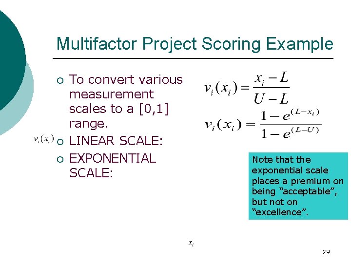
Multifactor Project Scoring Example ¡ ¡ ¡ To convert various measurement scales to a [0, 1] range. LINEAR SCALE: EXPONENTIAL SCALE: Note that the exponential scale places a premium on being “acceptable”, but not on “excellence”. 29

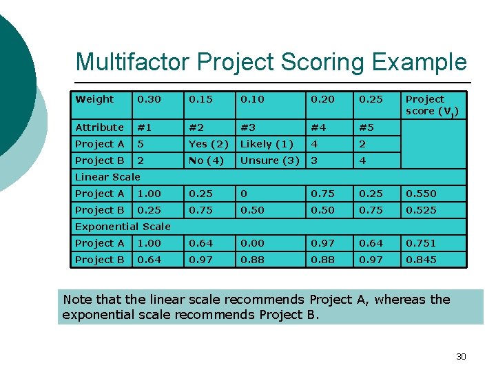
Multifactor Project Scoring Example Weight 0. 30 0. 15 0. 10 0. 25 Attribute #1 #2 #3 #4 #5 Project A 5 Yes (2) Likely (1) 4 2 Project B 2 No (4) Unsure (3) 3 4 Project score (Vj) Linear Scale Project A 1. 00 0. 25 0 0. 75 0. 25 0. 550 Project B 0. 25 0. 75 0. 50 0. 75 0. 525 Exponential Scale Project A 1. 00 0. 64 0. 00 0. 97 0. 64 0. 751 Project B 0. 64 0. 97 0. 88 0. 97 0. 845 Note that the linear scale recommends Project A, whereas the exponential scale recommends Project B. 30

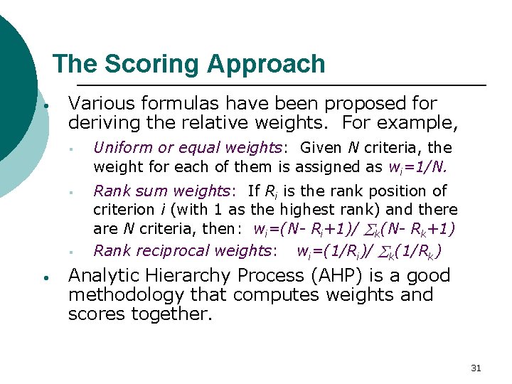
The Scoring Approach · · Various formulas have been proposed for deriving the relative weights. For example, § Uniform or equal weights: Given N criteria, the weight for each of them is assigned as wi=1/N. § Rank sum weights: If Ri is the rank position of criterion i (with 1 as the highest rank) and there are N criteria, then: wi=(N- Ri+1)/ k(N- Rk+1) § Rank reciprocal weights: wi=(1/Ri)/ k(1/Rk) Analytic Hierarchy Process (AHP) is a good methodology that computes weights and scores together. 31

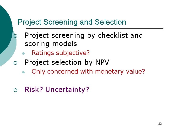
Project Screening and Selection ¡ Project screening by checklist and scoring models l ¡ Project selection by NPV l ¡ Ratings subjective? Only concerned with monetary value? Risk? Uncertainty? 32

Project selection using decision trees ¡ ¡ ¡ Decision trees are a powerful approach for decision making problems involving sequential decisions and variable outcomes over time. Project selection problem often involves uncertainties about the future. The outcomes of a project may change depending on which future scenario occurs. A decision tree is a graphical method of expressing the alternative actions that are available to the decision maker and the outcomes that may occur by chance. 33

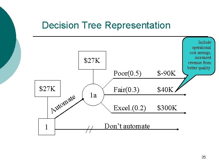
Project Selection by Decision Analysis § § Example - To determine whether a project to automate a manufacturing process should be launched or not. Depending on the extent of success of the project, the performance of the process after the automation project may turn out to be § § § poor, fair, or excellent. 34

Decision Tree Representation $27 K m o t u A 1 ate 1 a Poor(0. 5) $-90 K Fair(0. 3) $40 K Excel. (0. 2) $300 K Include operational cost savings, increased revenue from better quality. Don’t automate 35

Decision Analysis ¡ More about this topic later …. 36

Project Selection as a Portfolio Planning Problem ¡ ¡ ¡ A project is a multi-period investment problem. In each time period, the resources that are available, such as a budget to cover the costs of all projects in the portfolio, are limited. If the company is considering many (say 50 or 100) projects, the number of possible combinations of selected projects is huge. In order to select an “optimal” or even good combination, we need a methodology that can quickly and accurately compare all these possible combinations. The only methodology that can achieve this is 0 -1 programming, which can be implemented in Excel. Microsoft Project and other project management packages do not provide this capability. 37

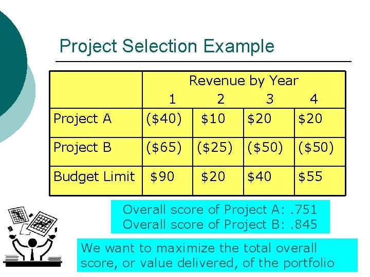
Project Selection Example Project A Revenue by Year 1 2 3 4 ($40) $10 $20 Project B ($65) ($25) $90 $20 Budget Limit ($50) $40 $55 Overall score of Project A: . 751 Overall score of Project B: . 845 We want to maximize the total overall score, or value delivered, of the portfolio 38

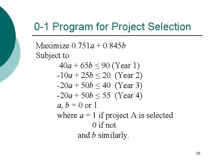
0 -1 Program for Project Selection Maximize 0. 751 a + 0. 845 b Subject to 40 a + 65 b ≤ 90 (Year 1) -10 a + 25 b ≤ 20 (Year 2) -20 a + 50 b ≤ 40 (Year 3) -20 a + 50 b ≤ 55 (Year 4) a, b = 0 or 1 where a = 1 if project A is selected 0 if not and b similarly. 39

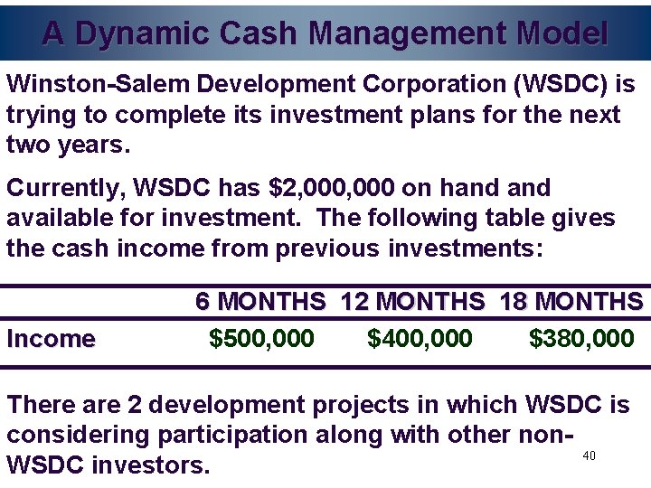
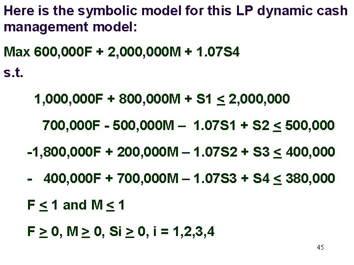
A Dynamic Cash Management Model Winston-Salem Development Corporation (WSDC) is trying to complete its investment plans for the next two years. Currently, WSDC has $2, 000 on hand available for investment. The following table gives the cash income from previous investments: Income 6 MONTHS 12 MONTHS 18 MONTHS $500, 000 $400, 000 $380, 000 There are 2 development projects in which WSDC is considering participation along with other non 40 WSDC investors.

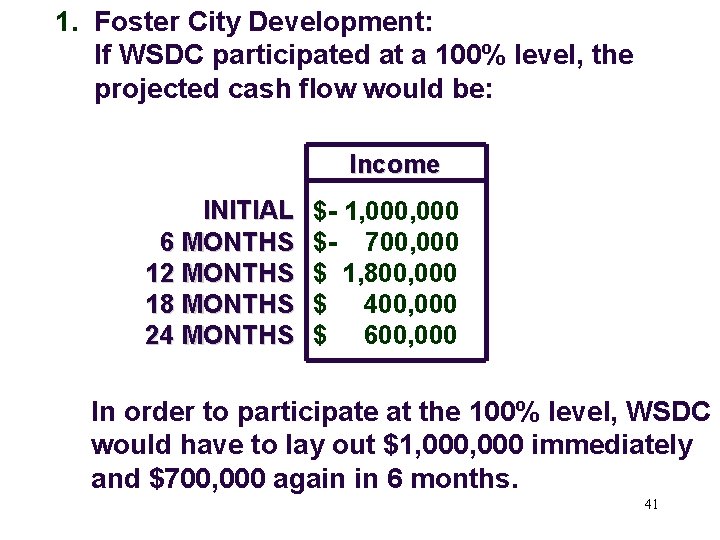
1. Foster City Development: If WSDC participated at a 100% level, the projected cash flow would be: Income INITIAL 6 MONTHS 12 MONTHS 18 MONTHS 24 MONTHS $- 1, 000 $- 700, 000 $ 1, 800, 000 $ 400, 000 $ 600, 000 In order to participate at the 100% level, WSDC would have to lay out $1, 000 immediately and $700, 000 again in 6 months. 41

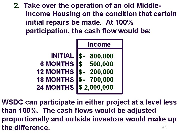
2. Take over the operation of an old Middle. Income Housing on the condition that certain initial repairs be made. At 100% participation, the cash flow would be: Income INITIAL 6 MONTHS 12 MONTHS 18 MONTHS 24 MONTHS $- 800, 000 $ 500, 000 $- 200, 000 $- 700, 000 $ 2, 000 WSDC can participate in either project at a level less than 100%. The cash flows would be adjusted proportionally and outside investors would make up 42 the difference.

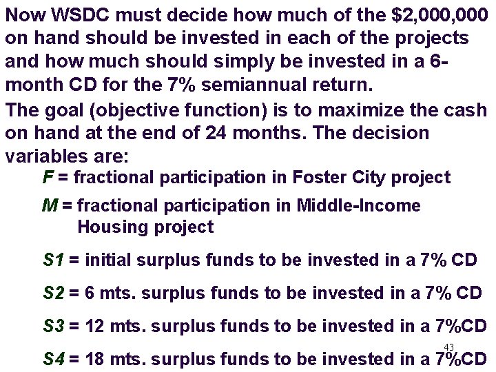
Now WSDC must decide how much of the $2, 000 on hand should be invested in each of the projects and how much should simply be invested in a 6 month CD for the 7% semiannual return. The goal (objective function) is to maximize the cash on hand at the end of 24 months. The decision variables are: F = fractional participation in Foster City project M = fractional participation in Middle-Income Housing project S 1 = initial surplus funds to be invested in a 7% CD S 2 = 6 mts. surplus funds to be invested in a 7% CD S 3 = 12 mts. surplus funds to be invested in a 7%CD 43 S 4 = 18 mts. surplus funds to be invested in a 7%CD

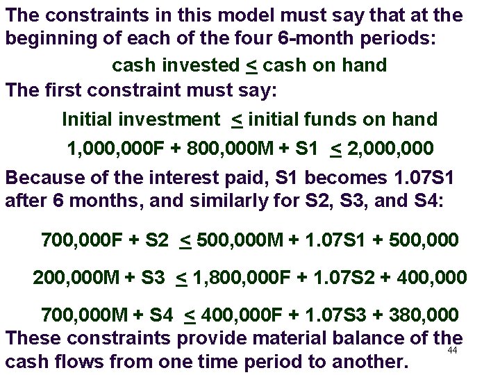
The constraints in this model must say that at the beginning of each of the four 6 -month periods: cash invested < cash on hand The first constraint must say: Initial investment < initial funds on hand 1, 000 F + 800, 000 M + S 1 < 2, 000 Because of the interest paid, S 1 becomes 1. 07 S 1 after 6 months, and similarly for S 2, S 3, and S 4: 700, 000 F + S 2 < 500, 000 M + 1. 07 S 1 + 500, 000 200, 000 M + S 3 < 1, 800, 000 F + 1. 07 S 2 + 400, 000 700, 000 M + S 4 < 400, 000 F + 1. 07 S 3 + 380, 000 These constraints provide material balance of the 44 cash flows from one time period to another.

Here is the symbolic model for this LP dynamic cash management model: Max 600, 000 F + 2, 000 M + 1. 07 S 4 s. t. 1, 000 F + 800, 000 M + S 1 < 2, 000 700, 000 F - 500, 000 M – 1. 07 S 1 + S 2 < 500, 000 -1, 800, 000 F + 200, 000 M – 1. 07 S 2 + S 3 < 400, 000 - 400, 000 F + 700, 000 M – 1. 07 S 3 + S 4 < 380, 000 F < 1 and M < 1 F > 0, M > 0, Si > 0, i = 1, 2, 3, 4 45

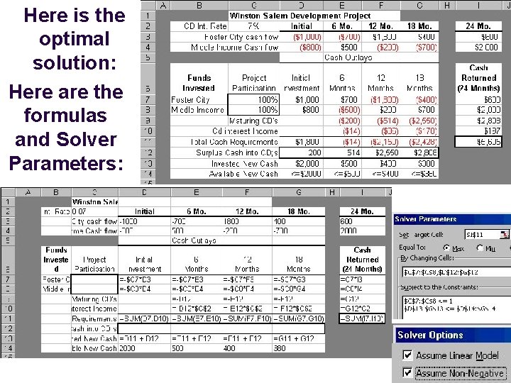
Here is the optimal solution: Here are the formulas and Solver Parameters: 46

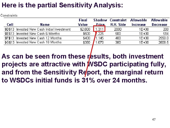
Here is the partial Sensitivity Analysis: As can be seen from these results, both investment projects are attractive with WSDC participating fully, and from the Sensitivity Report, the marginal return to WSDCs initial funds is 31% over 24 months. 47

Decision Support for Project Selection Tutorial on Linear Programming with Excel for Project Selection