Project ID PText 07 Optimum Operation in Power

Project ID: PT_ext 07 Optimum Operation in Power Distribution Systems Bachelor of Engineering (Honours) in Electrical Engineering Of The Hong Kong Polytechnic University Final Year Project Presentation By Student Name: IP SHING WAI Student ID: 14113295 D Supervisor: C. W. Yu

Flow of the presentation 1. Introduction 1. 1. Background 1. 2. Method of calculation of bus voltage 1. 3. Network Analysis 1. 4 Linear programming 1. 5. Dynamic programming method 2. Literature Review 3. Methodology ßStep 1. Data input ßStep 2. FDLF Method for calculation of bus voltage ßStep 3. Design by Network analysis ßStep 4. Dynamic Programming for searching optimal path 4. Finding/Results 4. 1. Allowable Switching Number Vs Power Loss 4. 2. Capacitors schedule for K=2 4. 3. Fixed schedule Vs Dynamic program (K=2) 4. 4. Power factor Vs Power loss 4. 5. Power Loss for variable location of capacitors 5. Conclusion and Recommendation 6. References

1. 1 Background Before: There still are fixed schedule control for capacitors dispatch Nowadays: Under monitoring system support, programming method can be used to design optimal schedule for capacitors control , including Dynamic programming

1. 1 Background (Cont) Unit Commitment (UC) Problem Given: ü 24 hour ü 4 capacitors control => (24)24 =7. 9228 x 1028 combination => Spend lots of time for calculation

1. 1 Background (Cont) Specific Objectives Study the optimal schedule of capacitors and power loss in power distribution with dynamic programming.

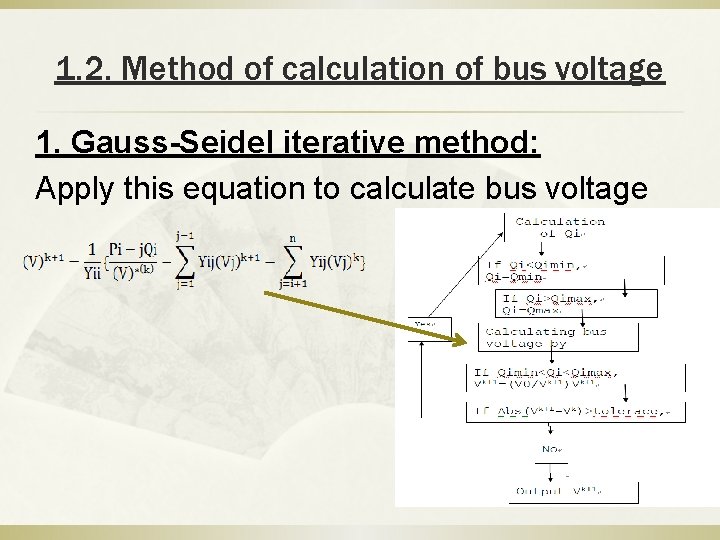
1. 2. Method of calculation of bus voltage 1. Gauss-Seidel iterative method: Apply this equation to calculate bus voltage

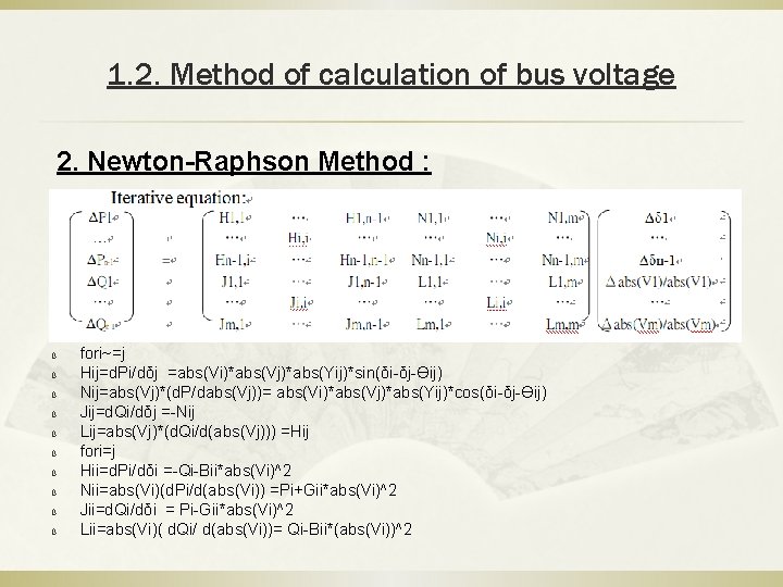
1. 2. Method of calculation of bus voltage 2. Newton-Raphson Method : ß ß ß ß ß fori~=j Hij=d. Pi/dδj =abs(Vi)*abs(Vj)*abs(Yij)*sin(δi-δj-Ɵij) Nij=abs(Vj)*(d. P/dabs(Vj))= abs(Vi)*abs(Vj)*abs(Yij)*cos(δi-δj-Ɵij) Jij=d. Qi/dδj =-Nij Lij=abs(Vj)*(d. Qi/d(abs(Vj))) =Hij fori=j Hii=d. Pi/dδi =-Qi-Bii*abs(Vi)^2 Nii=abs(Vi)(d. Pi/d(abs(Vi)) =Pi+Gii*abs(Vi)^2 Jii=d. Qi/dδi = Pi-Gii*abs(Vi)^2 Lii=abs(Vi)( d. Qi/ d(abs(Vi))= Qi-Bii*(abs(Vi))^2

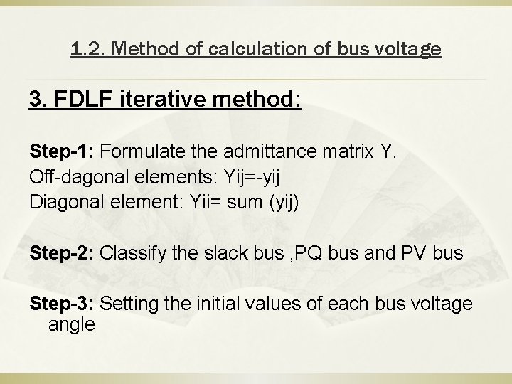
1. 2. Method of calculation of bus voltage 3. FDLF iterative method: Step-1: Formulate the admittance matrix Y. Off-dagonal elements: Yij=-yij Diagonal element: Yii= sum (yij) Step-2: Classify the slack bus , PQ bus and PV bus Step-3: Setting the initial values of each bus voltage angle

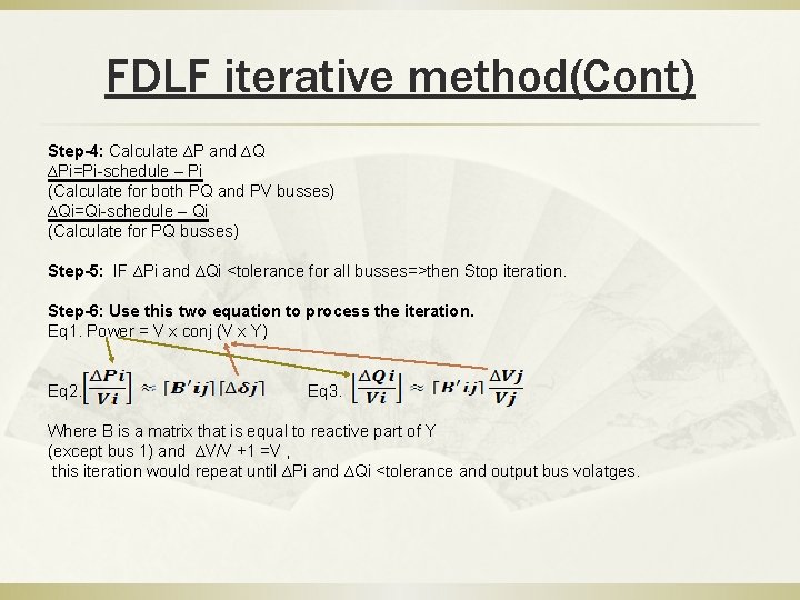
FDLF iterative method(Cont) Step-4: Calculate ∆P and ∆Q ∆Pi=Pi-schedule – Pi (Calculate for both PQ and PV busses) ∆Qi=Qi-schedule – Qi (Calculate for PQ busses) Step-5: IF ∆Pi and ∆Qi <tolerance for all busses=>then Stop iteration. Step-6: Use this two equation to process the iteration. Eq 1. Power = V x conj (V x Y) Eq 2. Eq 3. Where B is a matrix that is equal to reactive part of Y (except bus 1) and ∆V/V +1 =V , this iteration would repeat until ∆Pi and ∆Qi <tolerance and output bus volatges.

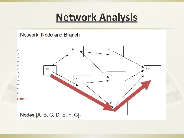
Network Analysis

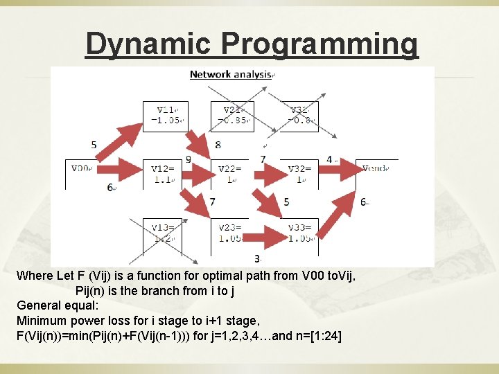
Dynamic Programming Where Let F (Vij) is a function for optimal path from V 00 to. Vij, Pij(n) is the branch from i to j General equal: Minimum power loss for i stage to i+1 stage, F(Vij(n))=min(Pij(n)+F(Vij(n-1))) for j=1, 2, 3, 4…and n=[1: 24]

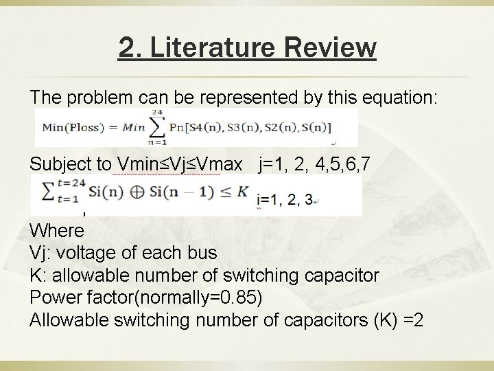
2. Literature Review The problem can be represented by this equation: Subject to Vmin≤Vj≤Vmax j=1, 2, 4, 5, 6, 7 Where Vj: voltage of each bus K: allowable number of switching capacitor Power factor(normally=0. 85) Allowable switching number of capacitors (K) =2

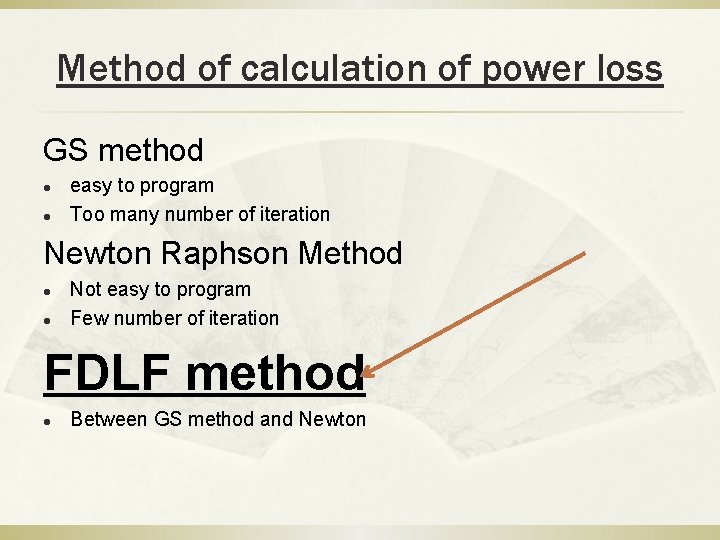
Method of calculation of power loss GS method l l easy to program Too many number of iteration Newton Raphson Method l l Not easy to program Few number of iteration FDLF method l Between GS method and Newton

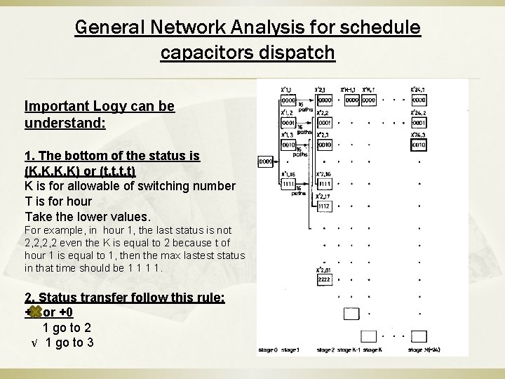
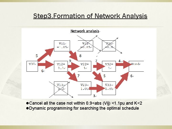
General Network Analysis for schedule capacitors dispatch Important Logy can be understand: 1. The bottom of the status is (K, K, K, K) or (t, t, t, t) K is for allowable of switching number T is for hour Take the lower values. For example, in hour 1, the last status is not 2, 2, 2, 2 even the K is equal to 2 because t of hour 1 is equal to 1, then the max lastest status in that time should be 1 1. 2. Status transfer follow this rule: +1 or +0 1 go to 2 √ 1 go to 3

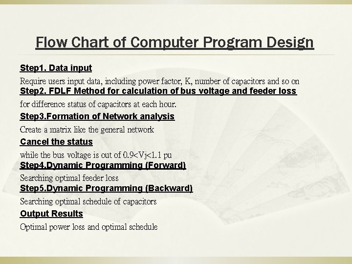
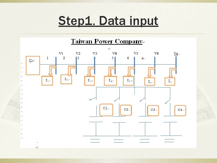
Flow Chart of Computer Program Design Step 1. Data input Require users input data, including power factor, K, number of capacitors and so on Step 2. FDLF Method for calculation of bus voltage and feeder loss for difference status of capacitors at each hour. Step 3. Formation of Network analysis Create a matrix like the general network Cancel the status while the bus voltage is out of 0. 9<Vj<1. 1 pu Step 4. Dynamic Programming (Forward) Searching optimal feeder loss Step 5. Dynamic Programming (Backward) Searching optimal schedule of capacitors Output Results Optimal power loss and optimal schedule

Step 1. Data input

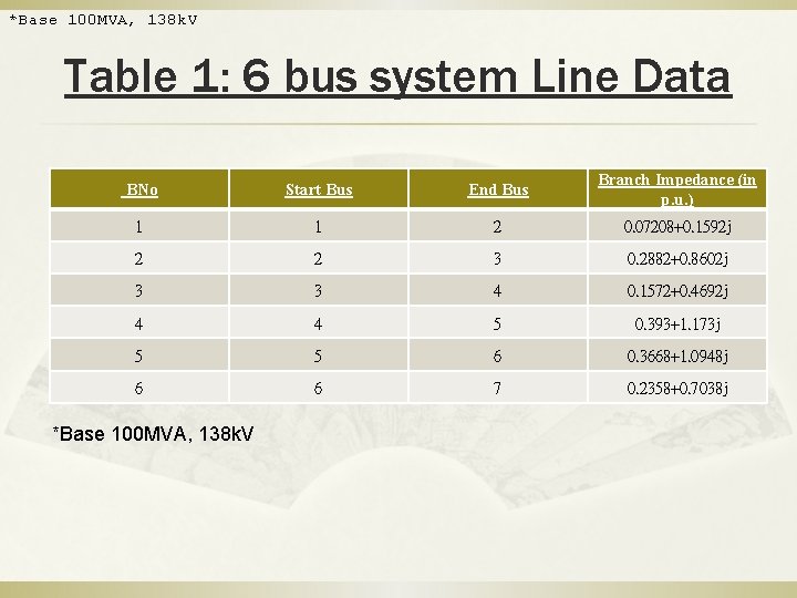
*Base 100 MVA, 138 k. V Table 1: 6 bus system Line Data BNo Start Bus End Bus Branch Impedance (in p. u. ) 1 1 2 0. 07208+0. 1592 j 2 2 3 0. 2882+0. 8602 j 3 3 4 0. 1572+0. 4692 j 4 4 5 0. 393+1. 173 j 5 5 6 0. 3668+1. 0948 j 6 6 7 0. 2358+0. 7038 j *Base 100 MVA, 138 k. V

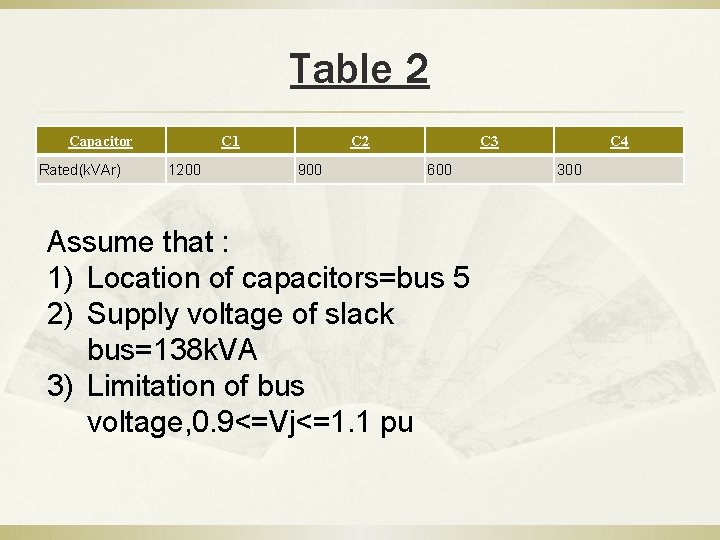
Table 2 Capacitor Rated(k. VAr) C 1 1200 C 2 900 C 3 600 Assume that : 1) Location of capacitors=bus 5 2) Supply voltage of slack bus=138 k. VA 3) Limitation of bus voltage, 0. 9<=Vj<=1. 1 pu C 4 300

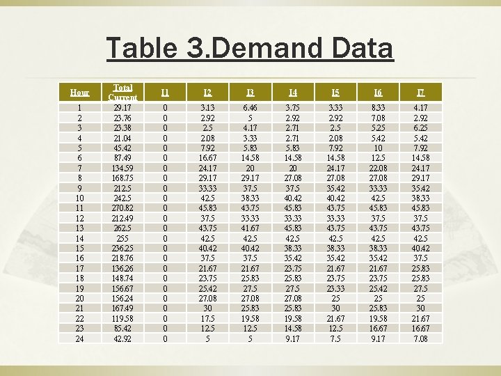
Table 3. Demand Data Hour 1 2 3 4 5 6 7 8 9 10 11 12 13 14 15 16 17 18 19 20 21 22 23 24 Total Current 29. 17 23. 76 23. 38 21. 04 45. 42 87. 49 134. 59 168. 75 212. 5 242. 5 270. 82 212. 49 262. 5 255 236. 25 218. 76 136. 26 148. 74 156. 67 156. 24 167. 49 119. 58 85. 42 42. 92 I 1 I 2 I 3 I 4 I 5 I 6 I 7 0 0 0 0 0 0 3. 13 2. 92 2. 5 2. 08 7. 92 16. 67 24. 17 29. 17 33. 33 42. 5 45. 83 37. 5 43. 75 42. 5 40. 42 37. 5 21. 67 23. 75 25. 42 27. 08 30 17. 5 12. 5 5 6. 46 5 4. 17 3. 33 5. 83 14. 58 20 29. 17 37. 5 38. 33 43. 75 33. 33 41. 67 42. 5 40. 42 37. 5 21. 67 25. 83 27. 5 27. 08 25. 83 19. 58 12. 5 5 3. 75 2. 92 2. 71 5. 83 14. 58 20 27. 08 37. 5 40. 42 45. 83 33. 33 45. 83 42. 5 38. 33 35. 42 23. 75 25. 83 27. 5 27. 08 25. 83 19. 58 14. 58 9. 17 3. 33 2. 92 2. 5 2. 08 7. 92 14. 58 24. 17 27. 08 35. 42 40. 42 43. 75 33. 33 43. 75 42. 5 38. 33 35. 42 21. 67 23. 75 23. 33 25 30 21. 67 12. 5 7. 5 8. 33 7. 08 5. 25 5. 42 10 12. 5 22. 08 27. 08 33. 33 42. 5 45. 83 37. 5 43. 75 42. 5 38. 33 35. 42 21. 67 23. 75 25. 42 25 25. 83 19. 58 16. 67 9. 17 4. 17 2. 92 6. 25 5. 42 7. 92 14. 58 24. 17 29. 17 35. 42 38. 33 45. 83 37. 5 43. 75 42. 5 40. 42 37. 5 25. 83 27. 5 25 30 21. 67 16. 67 7. 08

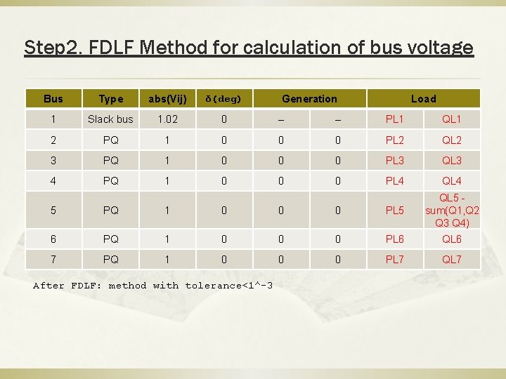
Step 2. FDLF Method for calculation of bus voltage Bus Type abs(Vij) δ(deg) 1 Slack bus 1. 02 0 -- -- PL 1 QL 1 2 PQ 1 0 0 0 PL 2 QL 2 3 PQ 1 0 0 0 PL 3 QL 3 4 PQ 1 0 0 0 PL 4 QL 4 Generation Load 5 PQ 1 0 0 0 PL 5 QL 5 sum(Q 1, Q 2 Q 3 Q 4) 6 PQ 1 0 0 0 PL 6 QL 6 7 PQ 1 0 0 0 PL 7 QL 7 After FDLF: method with tolerance<1^-3

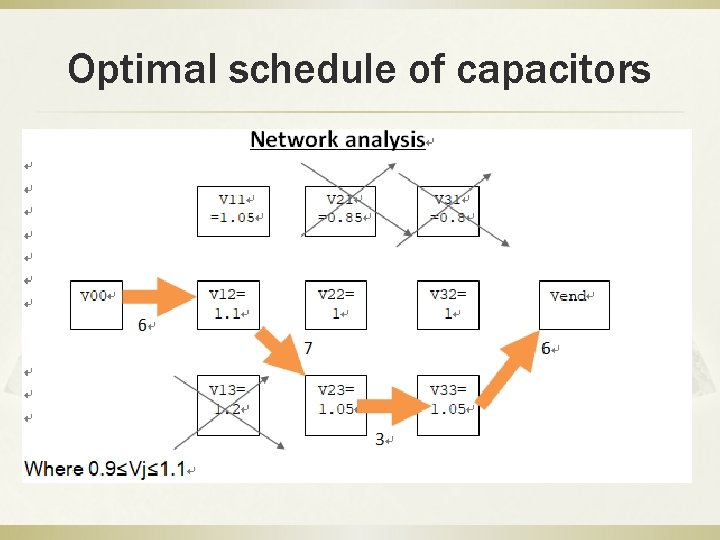
Step 3. Formation of Network Analysis l. Cancel all the case not within 0. 9<abs (Vij) <1. 1 pu and K<2 l. Dynamic programming for searching the optimal schedule

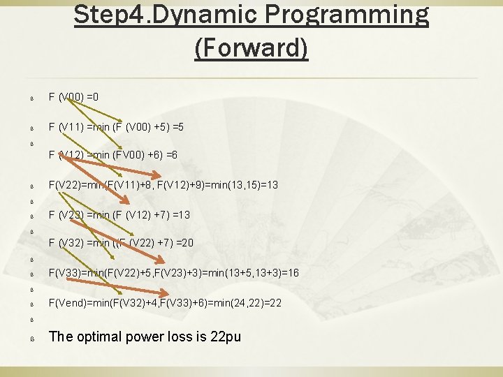
Step 4. Dynamic Programming (Forward) ß F (V 00) =0 ß F (V 11) =min (F (V 00) +5) =5 ß F (V 12) =min (FV 00) +6) =6 ß F(V 22)=min(F(V 11)+8, F(V 12)+9)=min(13, 15)=13 ß ß F (V 23) =min (F (V 12) +7) =13 ß F (V 32) =min ((F (V 22) +7) =20 ß ß F(V 33)=min(F(V 22)+5, F(V 23)+3)=min(13+5, 13+3)=16 ß ß F(Vend)=min(F(V 32)+4, F(V 33)+6)=min(24, 22)=22 ß ß The optimal power loss is 22 pu

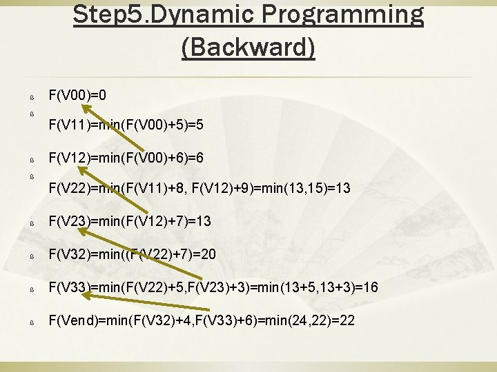
Step 5. Dynamic Programming (Backward) ß ß F(V 00)=0 F(V 11)=min(F(V 00)+5)=5 F(V 12)=min(F(V 00)+6)=6 F(V 22)=min(F(V 11)+8, F(V 12)+9)=min(13, 15)=13 ß F(V 23)=min(F(V 12)+7)=13 ß F(V 32)=min((F(V 22)+7)=20 ß F(V 33)=min(F(V 22)+5, F(V 23)+3)=min(13+5, 13+3)=16 ß F(Vend)=min(F(V 32)+4, F(V 33)+6)=min(24, 22)=22

Optimal schedule of capacitors

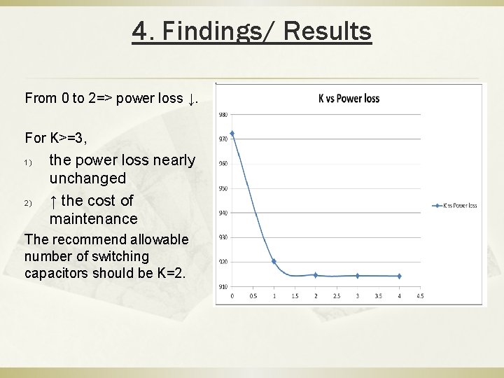
4. Findings/ Results From 0 to 2=> power loss ↓. For K>=3, 1) 2) the power loss nearly unchanged ↑ the cost of maintenance The recommend allowable number of switching capacitors should be K=2.

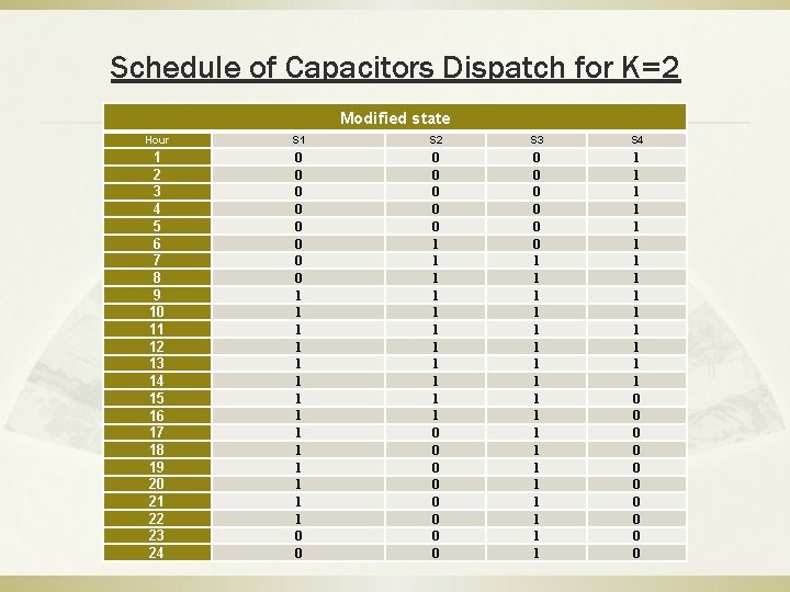
Schedule of Capacitors Dispatch for K=2 Modified state Hour S 1 S 2 S 3 S 4 1 2 3 4 5 6 7 8 9 10 11 12 13 14 15 16 17 18 19 20 21 22 23 24 0 0 0 0 1 1 1 1 0 0 0 0 1 1 1 0 0 0 0 1 1 1 1 1 1 1 1 0 0 0 0 0

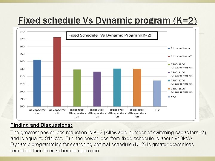
Fixed schedule Vs Dynamic program (K=2) Finding and Discussions: The greatest power loss reduction is K=2 (Allowable number of switching capacitors=2) and is equal to 914 k. VA. But, the power loss from fixed schedule is about 940 k. VA. Dynamic programming for searching optimal schedule (K=2) is greater power loss reduction than fixed schedule operation.

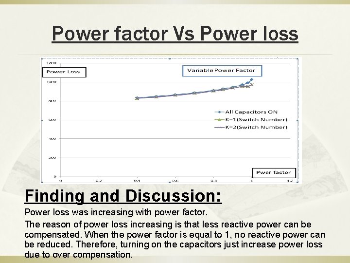
Power factor Vs Power loss Finding and Discussion: Power loss was increasing with power factor. The reason of power loss increasing is that less reactive power can be compensated. When the power factor is equal to 1, no reactive power can be reduced. Therefore, turning on the capacitors just increase power loss due to over compensation.

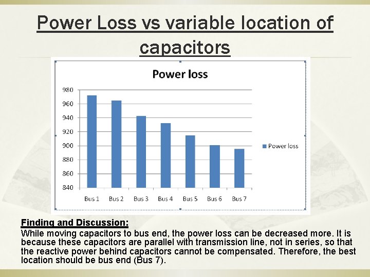
Power Loss vs variable location of capacitors Finding and Discussion: While moving capacitors to bus end, the power loss can be decreased more. It is because these capacitors are parallel with transmission line, not in series, so that the reactive power behind capacitors cannot be compensated. Therefore, the best location should be bus end (Bus 7).

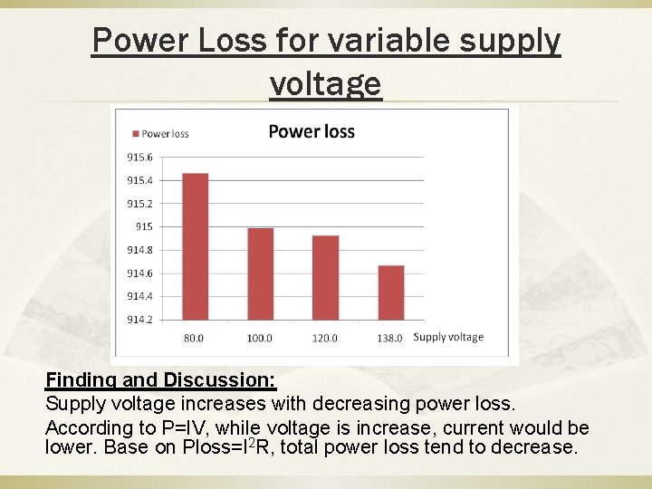
Power Loss for variable supply voltage Finding and Discussion: Supply voltage increases with decreasing power loss. According to P=IV, while voltage is increase, current would be lower. Base on Ploss=I 2 R, total power loss tend to decrease.

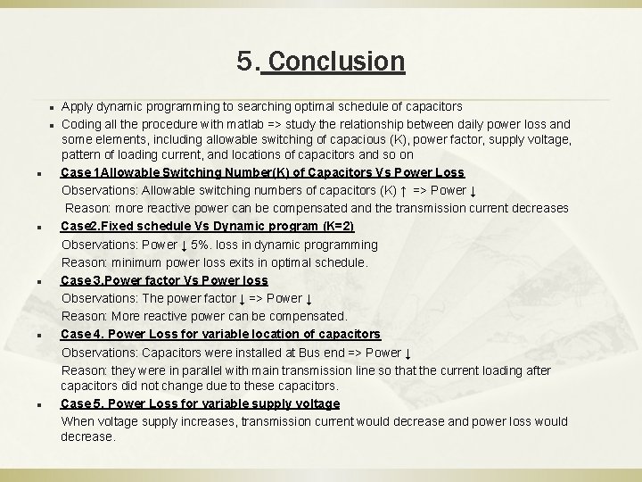
5. Conclusion l l l l Apply dynamic programming to searching optimal schedule of capacitors Coding all the procedure with matlab => study the relationship between daily power loss and some elements, including allowable switching of capacious (K), power factor, supply voltage, pattern of loading current, and locations of capacitors and so on Case 1 Allowable Switching Number(K) of Capacitors Vs Power Loss Observations: Allowable switching numbers of capacitors (K) ↑ => Power ↓ Reason: more reactive power can be compensated and the transmission current decreases Case 2. Fixed schedule Vs Dynamic program (K=2) Observations: Power ↓ 5%. loss in dynamic programming Reason: minimum power loss exits in optimal schedule. Case 3. Power factor Vs Power loss Observations: The power factor ↓ => Power ↓ Reason: More reactive power can be compensated. Case 4. Power Loss for variable location of capacitors Observations: Capacitors were installed at Bus end => Power ↓ Reason: they were in parallel with main transmission line so that the current loading after capacitors did not change due to these capacitors. Case 5. Power Loss for variable supply voltage When voltage supply increases, transmission current would decrease and power loss would decrease.

6. References 1. R. Bronson and G. Naadimuthu, Schaum's outline of theory and problems of Operations. Research, Mc. Graw Hill, 1997) Chapter 1. Mathematical Programming, pp. 1 ~ 7. Chapter 2. Linear Programming: Basic Concepts, pp. 18 ~ 20. Chapter 13. Network Analysis, pp. 216 ~ 227. 2. Frederick s. Hillier and Gerald J. Lieberman, Introduction to Operations. Research. Eighth Edition, Mc. Graw Hill, 2000 Chapter 9. Network Optimization Models, pp. 374 ~ 396. 3. Y. Y. Hsu, Ph. D and H-C. Kuo, MSc, Dispatch of capacitors on distribution system using dynamic programming, IEE PROCEEDING-C, Vol. 140, No. 6, November 1993 Power Generation Operation and Control’ by Allen J. Wood and B. F. Wollenberg (page 72 -79) 4. IEEE (http: //ieeexplore. ieee. org/document/1295033/) 5. You. Tube(https: //www. youtube. com/watch? v=t. GQPZz. Fb. LPE CEATI (https: //www. ceati. com/collaborative-programs/transmission-distribution/pspo-power-system-planning-operations/) 6. WIKI(https: //en. wikipedia. org/wiki/Unit_commitment_problem_in_electrical_power_production) 7. You. Tube(https: //www. youtube. com/watch? v=t. GQPZz. Fb. LPE 8. CEATI (https: //www. ceati. com/collaborative-programs/transmission-distribution/pspo-power-system-planning-operations/) 9. WIKI(https: //en. wikipedia. org/wiki/Unit_commitment_problem_in_electrical_power_production)

ENG