Project 2 Presentation Spatial Databases GIS Case Studies

Project 2 Presentation Spatial Databases GIS Case Studies Elizabeth Sayed Elizabeth Stoltzfus December 4, 2002 UC Berkeley: IEOR 215

Agenda 4 Spatial Database Basics 4 Geographic Information Systems (GIS) Basics 4 Case Studies UC Berkeley: IEOR 215 1

Spatial Database Basics 4 Common applications UC Berkeley: IEOR 215 2

Spatial Databases Background 4 Spatial databases provide structures for storage and analysis of spatial data 4 Spatial data is comprised of objects in multi-dimensional space 4 Storing spatial data in a standard database would require excessive amounts of space 4 Queries to retrieve and analyze spatial data from a standard database would be long and cumbersome leaving a lot of room for error 4 Spatial databases provide much more efficient storage, retrieval, and analysis of spatial data UC Berkeley: IEOR 215 3

Types of Data Stored in Spatial Databases 4 Two-dimensional data examples – Geographical – Cartesian coordinates (2 -D) – Networks – Direction 4 Three-dimensional data examples – Weather – Cartesian coordinates (3 -D) – Topological – Satellite images UC Berkeley: IEOR 215 4

Spatial Databases Uses and Users 4 Three types of uses – Manage spatial data – Analyze spatial data – High level utilization 4 A few examples of users – Transportation agency tracking projects – Insurance risk manager considering location risk profiles – Doctor comparing Magnetic Resonance Images (MRIs) – Emergency response determining quickest route to victim – Mobile phone companies tracking phone usage UC Berkeley: IEOR 215 5

Spatial Databases Uses and Users 4 Three types of uses – Manage spatial data – Analyze spatial data – High level utilization 4 A few examples of users – Transportation agency tracking projects – Insurance risk manager considering location risk profiles – Doctor comparing Magnetic Resonance Images (MRIs) – Emergency response determining quickest route to victim – Mobile phone user determining current relative location of businesses UC Berkeley: IEOR 215 6

Spatial Database Management System 4 Spatial Database Management System (SDBMS) provides the capabilities of a traditional database management system (DBMS) while allowing special storage and handling of spatial data. 4 SDBMS: – Works with an underlying DBMS – Allows spatial data models and types – Supports querying language specific to spatial data types – Provides handling of spatial data and operations UC Berkeley: IEOR 215 7

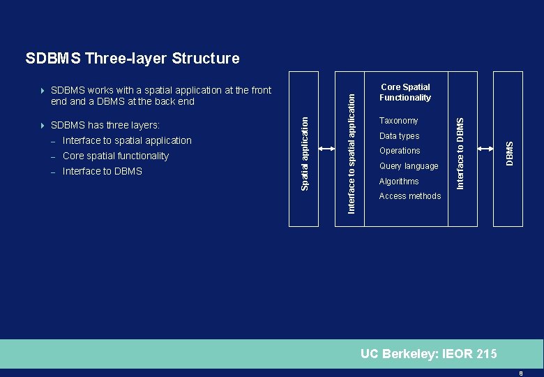
Interface to spatial application – Core spatial functionality – Interface to DBMS Taxonomy Data types Operations Query language Algorithms DBMS – Core Spatial Functionality Interface to DBMS 4 SDBMS has three layers: Spatial application 4 SDBMS works with a spatial application at the front end a DBMS at the back end Interface to spatial application SDBMS Three-layer Structure Access methods UC Berkeley: IEOR 215 8

Spatial Query Language 4 Number of specialized adaptations of SQL – Spatial query language – Temporal query language (TSQL 2) – Object query language (OQL) – Object oriented structured query language (O 2 SQL) 4 Spatial query language provides tools and structures specifically for working with spatial data 4 SQL 3 provides 2 D geospatial types and functions UC Berkeley: IEOR 215 9

Spatial Query Language Operations 4 Three types of queries: – Basic operations on all data types (e. g. Is. Empty, Envelope, Boundary) – Topological/set operators (e. g. Disjoint, Touch, Contains) – Spatial analysis (e. g. Distance, Intersection, Symm. Diff) UC Berkeley: IEOR 215 10

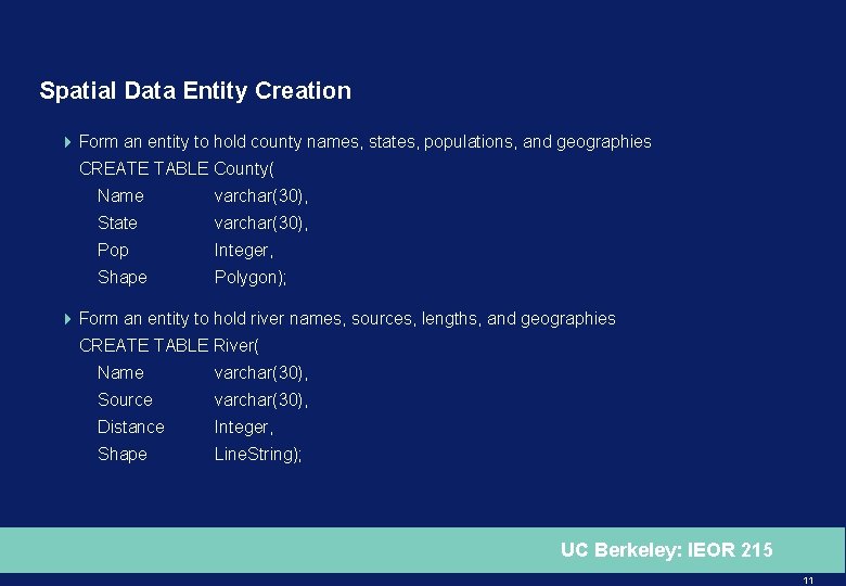
Spatial Data Entity Creation 4 Form an entity to hold county names, states, populations, and geographies CREATE TABLE County( Name varchar(30), State varchar(30), Pop Integer, Shape Polygon); 4 Form an entity to hold river names, sources, lengths, and geographies CREATE TABLE River( Name varchar(30), Source varchar(30), Distance Integer, Shape Line. String); UC Berkeley: IEOR 215 11

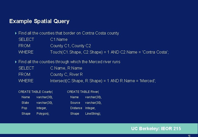
Example Spatial Query 4 Find all the counties that border on Contra Costa county SELECT C 1. Name FROM County C 1, County C 2 WHERE Touch(C 1. Shape, C 2. Shape) = 1 AND C 2. Name = ‘Contra Costa’; 4 Find all the counties through which the Merced river runs SELECT C. Name, R. Name FROM County C, River R WHERE Intersect(C. Shape, R. Shape) = 1 AND R. Name = ‘Merced’; CREATE TABLE County( CREATE TABLE River( Name varchar(30), State varchar(30), Source varchar(30), Pop Integer, Distance Integer, Shape Polygon); Shape Line. String); UC Berkeley: IEOR 215 12

Geographic Information System (GIS) Basics 4 Common applications UC Berkeley: IEOR 215 13

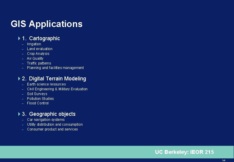
GIS Applications 41. Cartographic – – – Irrigation Land evaluation Crop Analysis Air Quality Traffic patterns Planning and facilities management 42. Digital Terrain Modeling – – – Earth science resources Civil Engineering & Military Evaluation Soil Surveys Pollution Studies Flood Control 43. Geographic objects – – – Car navigation systems Utility distribution and consumption Consumer product and services UC Berkeley: IEOR 215 14

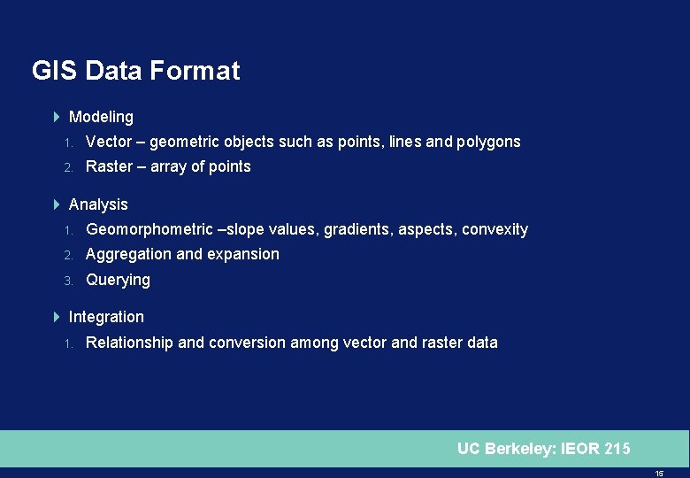
GIS Data Format 4 Modeling 1. Vector – geometric objects such as points, lines and polygons 2. Raster – array of points 4 Analysis 1. Geomorphometric –slope values, gradients, aspects, convexity 2. Aggregation and expansion 3. Querying 4 Integration 1. Relationship and conversion among vector and raster data UC Berkeley: IEOR 215 15

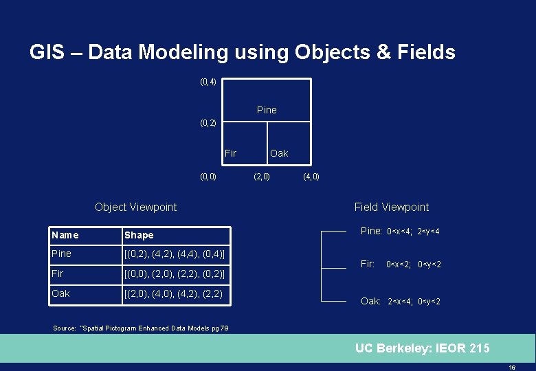
GIS – Data Modeling using Objects & Fields (0, 4) Pine (0, 2) Fir (0, 0) Object Viewpoint Name Shape Pine [(0, 2), (4, 4), (0, 4)] Fir [(0, 0), (2, 2), (0, 2)] Oak [(2, 0), (4, 2), (2, 2) Oak (2, 0) (4, 0) Field Viewpoint Pine: 0<x<4; 2<y<4 Fir: 0<x<2; 0<y<2 Oak: 2<x<4; 0<y<2 Source: “Spatial Pictogram Enhanced Data Models pg 79 UC Berkeley: IEOR 215 16

Conceptual Data Modeling 4 Relational Databases: ER diagram 4 Limitations for ER with respect to Spatial databases: – Can not capture semantics – No notion of key attributes and unique OID’s in a field model – ER Relationship between entities derived from application under consideration – Spatial Relationships are inherent between objects 4 Solution: Pictograms for Spatial Conceptual Data-Modeling UC Berkeley: IEOR 215 17

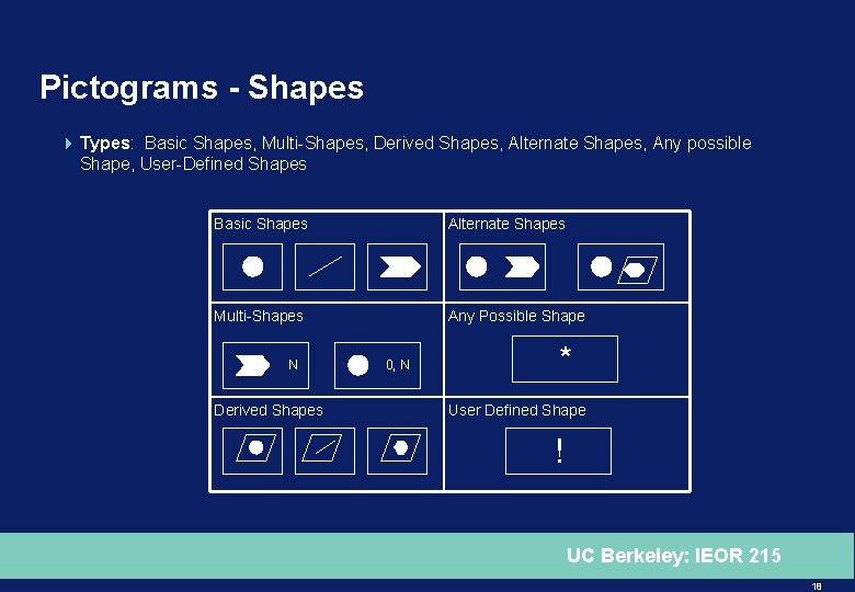
Pictograms - Shapes 4 Types: Basic Shapes, Multi-Shapes, Derived Shapes, Alternate Shapes, Any possible Shape, User-Defined Shapes Basic Shapes Alternate Shapes Multi-Shapes Any Possible Shape N Derived Shapes 0, N * User Defined Shape ! UC Berkeley: IEOR 215 18

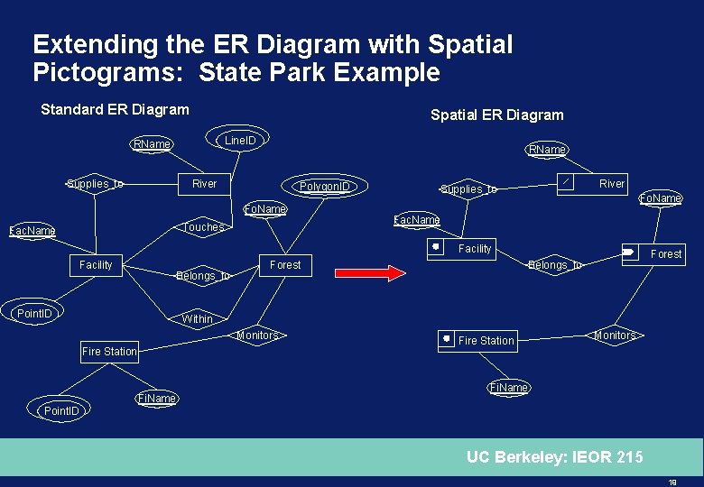
Extending the ER Diagram with Spatial Pictograms: State Park Example Standard ER Diagram Spatial ER Diagram Line. ID RName River Supplies_to Polygon. ID Fo. Name Touches Fac. Name River Supplies_to Fo. Name Facility Belongs_to Point. ID Forest Belongs_to Within Monitors Fire Station Fi. Name Fire Station Monitors Fi. Name Point. ID UC Berkeley: IEOR 215 19

Case Studies 4 Specific applications of spatial databases UC Berkeley: IEOR 215 20

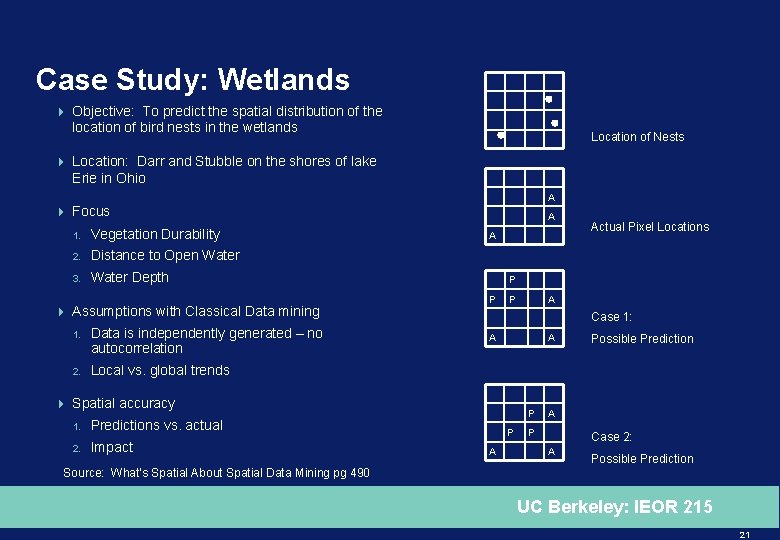
Case Study: Wetlands 4 Objective: To predict the spatial distribution of the location of bird nests in the wetlands Location of Nests 4 Location: Darr and Stubble on the shores of lake Erie in Ohio A 4 Focus 1. Vegetation Durability 2. Distance to Open Water 3. Water Depth 4 Assumptions with Classical Data mining 1. Data is independently generated – no autocorrelation 2. Local vs. global trends A A P Predictions vs. actual 2. Impact A Case 1: A A 4 Spatial accuracy 1. Actual Pixel Locations P P A Possible Prediction A P Case 2: A Possible Prediction Source: What’s Spatial About Spatial Data Mining pg 490 UC Berkeley: IEOR 215 21

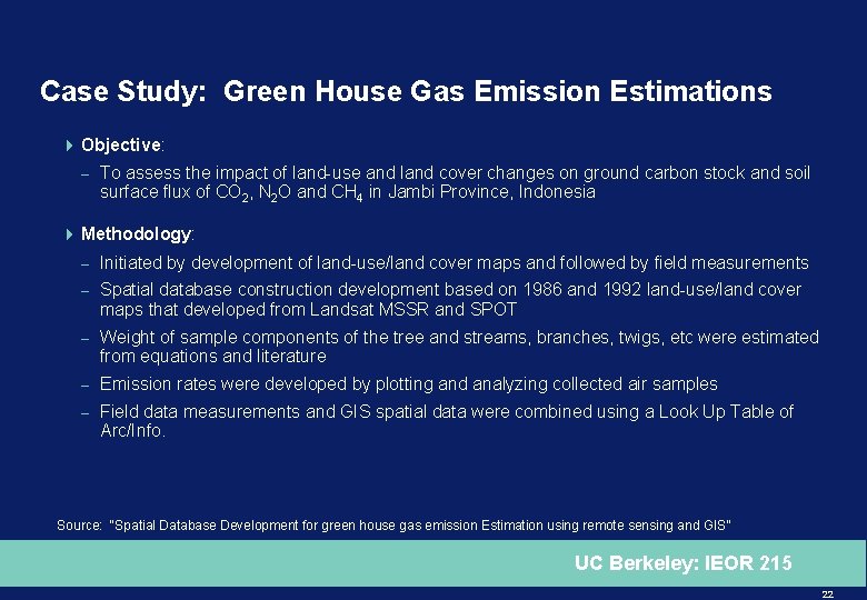
Case Study: Green House Gas Emission Estimations 4 Objective: – To assess the impact of land-use and land cover changes on ground carbon stock and soil surface flux of CO 2, N 2 O and CH 4 in Jambi Province, Indonesia 4 Methodology: – Initiated by development of land-use/land cover maps and followed by field measurements – Spatial database construction development based on 1986 and 1992 land-use/land cover maps that developed from Landsat MSSR and SPOT – Weight of sample components of the tree and streams, branches, twigs, etc were estimated from equations and literature – Emission rates were developed by plotting and analyzing collected air samples – Field data measurements and GIS spatial data were combined using a Look Up Table of Arc/Info. Source: “Spatial Database Development for green house gas emission Estimation using remote sensing and GIS” UC Berkeley: IEOR 215 22

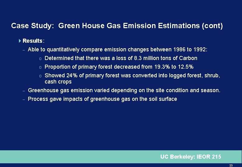
Case Study: Green House Gas Emission Estimations (cont) 4 Results: – Able to quantitatively compare emission changes between 1986 to 1992: o Determined that there was a loss of 8. 3 million tons of Carbon o Proportion of primary forest decreased from 19. 3% to 12. 5% o Showed 24% of primary forest was converted into logged forest, shrub, cash crops – Greenhouse gas emission varied depending on the site condition and season. – Process gave impacts of greenhouse gas on the soil surface UC Berkeley: IEOR 215 23

Case Study: Pantanal Area, Brazil 4 Objective: To assess the drastic land use changes in the Pantanal region since 1985 4 Data Source: – 3 Landsat TM images of the Pantal study area from 1985, 1990, 1996 – A land-use survey from 1997 4 Assessment Methodology: – Normalized Difference Vegetation Index (NDVI) was computed for each year – NDVI maps of the three years combined and submitted to multi-dimensional image segmentation – Classified vegetation – Produced a color composite by year that identified the density of vegetation Source: Integrated Spatial Databases pg 116 UC Berkeley: IEOR 215 24

Conclusion 4 Many varied applications of spatial databases 4 Stores spatial data in various formats specific to use 4 Captures spatial data more concisely 4 Enables more thorough understanding of data 4 Retrieves and manipulates spatial data more efficiently and effectively UC Berkeley: IEOR 215 25

UC Berkeley: IEOR 215 26

Problem 1 Solution a) Find all cities that are located within Marin County. SELECT C 2. Name FROM County C 1, City C 2 WHERE Within(C 1. Shape, C 2. Shape) = 1 AND C 1. Name = ‘Marin’; b) Find any rivers that borders on Mendocino County. SELECT R. Name FROM County C, River R WHERE Touch(C. Shape, R. Shape) = 1 AND C. Name = ‘Mendocino’; c) Find the counties that do not touch on Orange County. SELECT C 1. Name FROM County C 1, County C 2 WHERE Disjoint(C 1. Shape, C 2. Shape) = 1 AND C 2. Name = ‘Orange’; UC Berkeley: IEOR 215 27

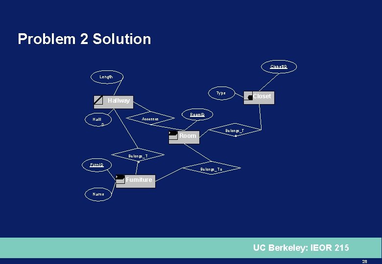
Problem 2 Solution Closet. ID Length Type Hallway Closet Room. ID Accesses Hall. I D Belongs_T o Room Belongs_T Furn. ID o Belongs_To Furniture Name UC Berkeley: IEOR 215 28