Project 1 Brake System Modelling Control Objective To

Project 1: Brake System Modelling & Control

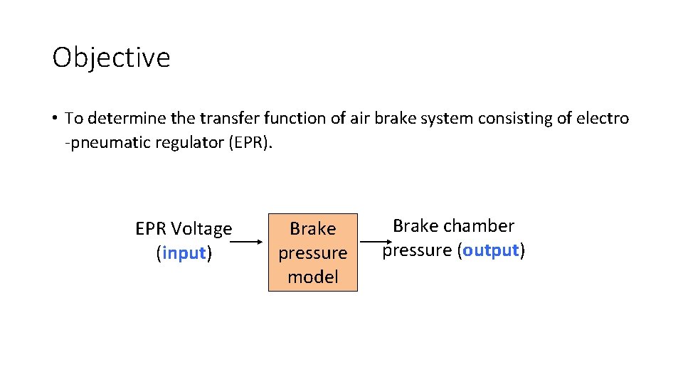
Objective • To determine the transfer function of air brake system consisting of electro -pneumatic regulator (EPR). EPR Voltage (input) Brake pressure model Brake chamber pressure (output)

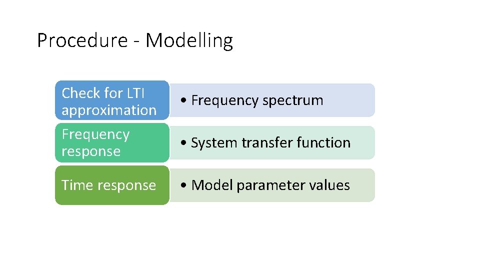
Procedure - Modelling Check for LTI approximation Frequency response Time response • Frequency spectrum • System transfer function • Model parameter values

Check for LTI – Spectral analysis • This method feeds a sinusoidal input voltage to the system and analyses the frequency content in the output.

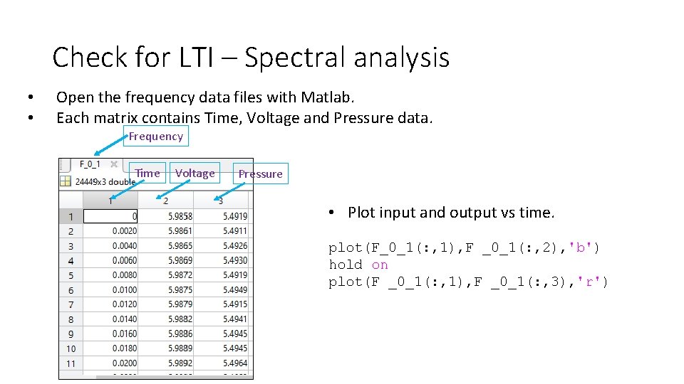
Check for LTI – Spectral analysis • • Open the frequency data files with Matlab. Each matrix contains Time, Voltage and Pressure data. Frequency Time Voltage Pressure • Plot input and output vs time. plot(F_0_1(: , 1), F _0_1(: , 2), 'b') hold on plot(F _0_1(: , 1), F _0_1(: , 3), 'r')

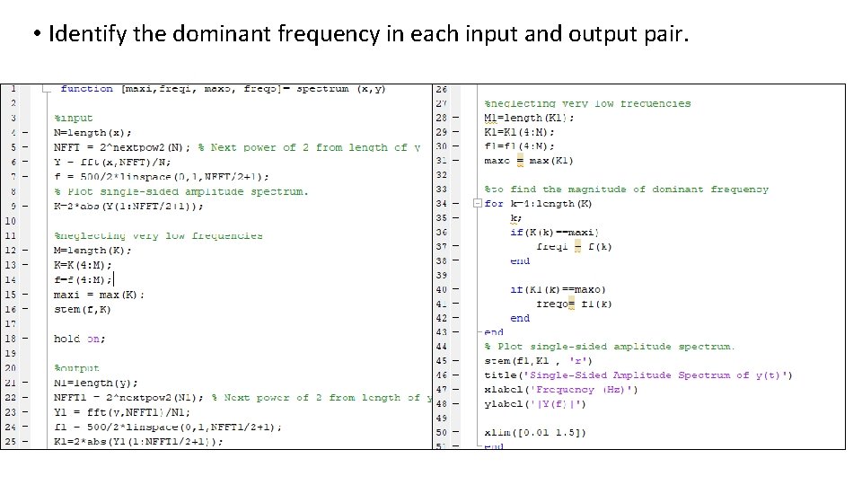
• Identify the dominant frequency in each input and output pair.

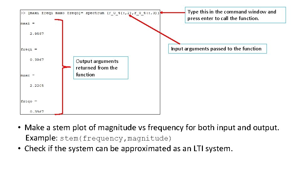
Type this in the command window and press enter to call the function. Input arguments passed to the function Output arguments returned from the function • Make a stem plot of magnitude vs frequency for both input and output. Example: stem(frequency, magnitude) • Check if the system can be approximated as an LTI system.

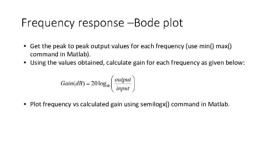
Frequency response –Bode plot • Get the peak to peak output values for each frequency (use min() max() command in Matlab). • Using the values obtained, calculate gain for each frequency as given below: • Plot frequency vs calculated gain using semilogx() command in Matlab.

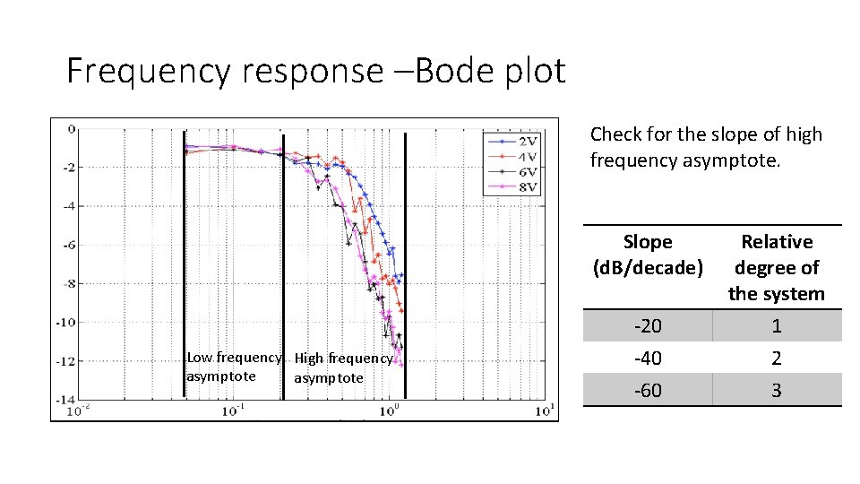
Frequency response –Bode plot Check for the slope of high frequency asymptote. Slope (d. B/decade) Low frequency High frequency asymptote -20 -40 -60 Relative degree of the system 1 2 3

Transfer Function Structure Using Pade’s Approximation, Model values to be found

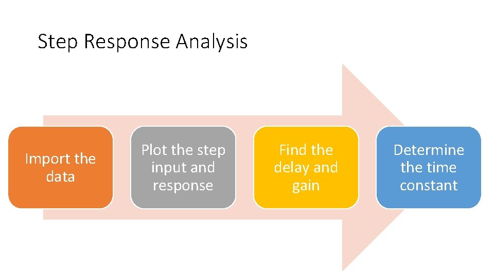
Step Response Analysis Import the data Plot the step input and response Find the delay and gain Determine the time constant

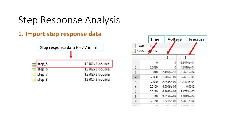
Step Response Analysis 1. Import step response data Step response data for 5 V input Time Voltage Pressure

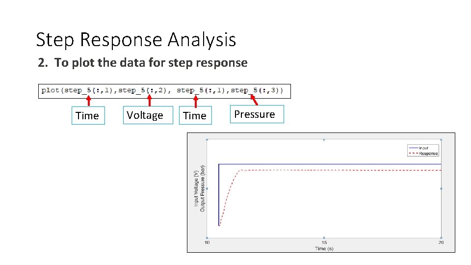
Step Response Analysis 2. To plot the data for step response Time Voltage Time Pressure

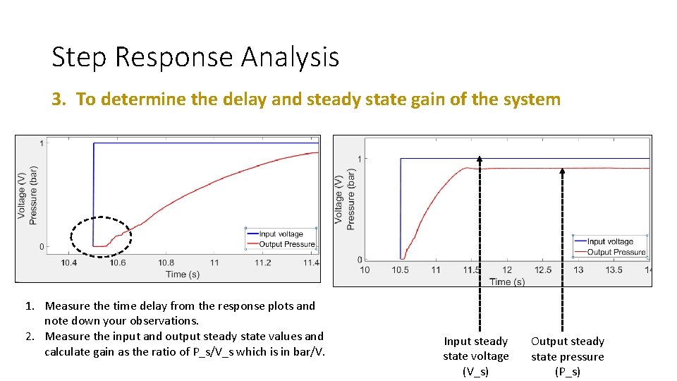
Step Response Analysis 3. To determine the delay and steady state gain of the system 1. Measure the time delay from the response plots and note down your observations. 2. Measure the input and output steady state values and calculate gain as the ratio of P_s/V_s which is in bar/V. Input steady state voltage (V_s) Output steady state pressure (P_s)

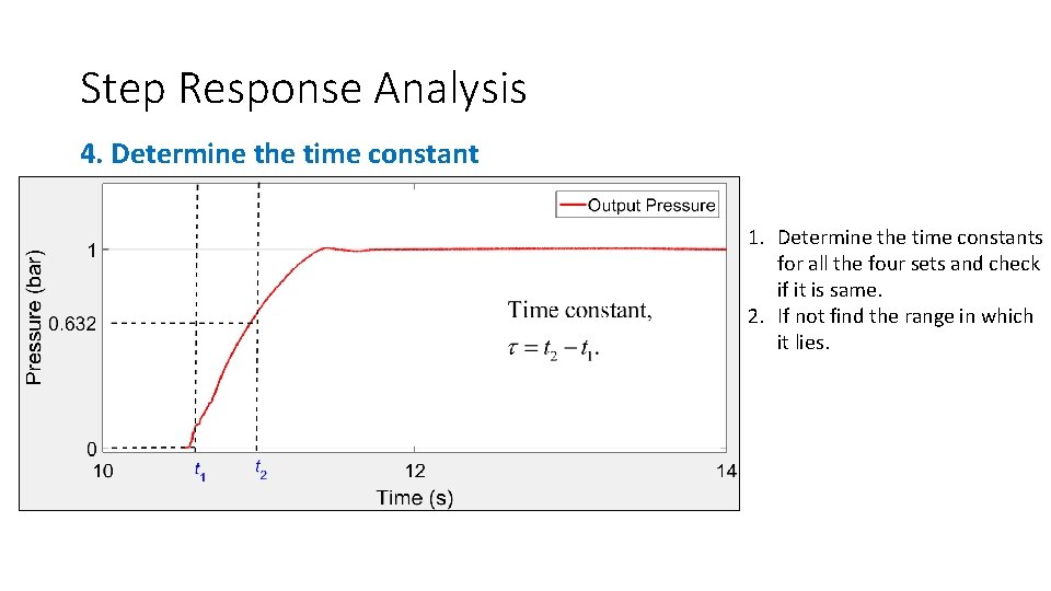
Step Response Analysis 4. Determine the time constant 1. Determine the time constants for all the four sets and check if it is same. 2. If not find the range in which it lies.

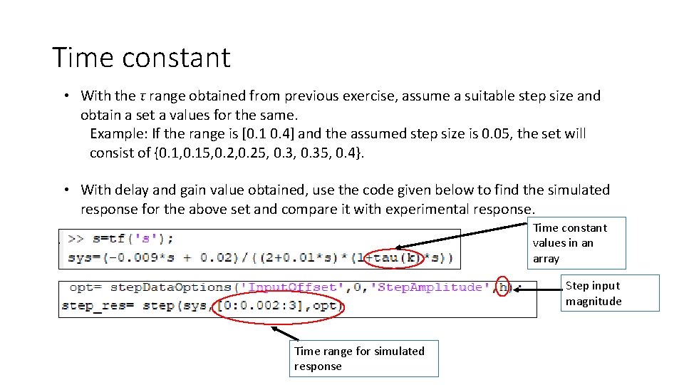
Time constant • With the τ range obtained from previous exercise, assume a suitable step size and obtain a set a values for the same. Example: If the range is [0. 1 0. 4] and the assumed step size is 0. 05, the set will consist of {0. 1, 0. 15, 0. 25, 0. 35, 0. 4}. • With delay and gain value obtained, use the code given below to find the simulated response for the above set and compare it with experimental response. Time constant values in an array Step input magnitude Time range for simulated response

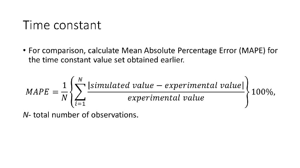
Time constant •

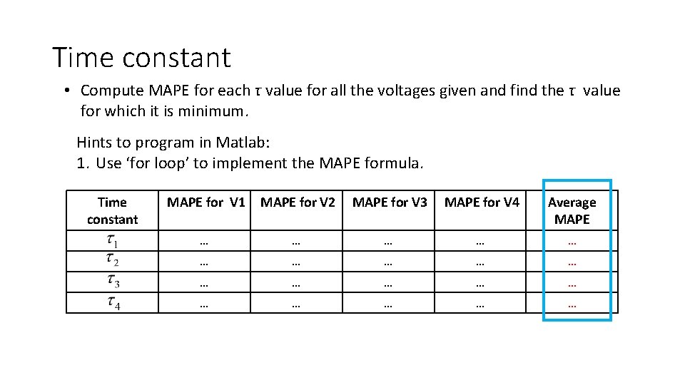
Time constant • Compute MAPE for each τ value for all the voltages given and find the τ value for which it is minimum. Hints to program in Matlab: 1. Use ‘for loop’ to implement the MAPE formula. Time constant MAPE for V 1 MAPE for V 2 MAPE for V 3 MAPE for V 4 Average MAPE … … … … …

Gdrive link https: //drive. google. com/file/d/1 C 39 m. Dgku 0 anc 0 vufnh. Kz. Kuu. Yia. A 24 F Cb/view? usp=sharing