Progress in Unstructured Mesh Techniques Dimitri J Mavriplis

Progress in Unstructured Mesh Techniques Dimitri J. Mavriplis Department of Mechanical Engineering University of Wyoming and Scientific Simulations Laramie, WY

Overview • NSU 3 D Unstructured Multigrid Navier-Stokes Solver – 2 nd order finite-volume discretization – Fast steady state solutions • (~100 M pts in 15 minutes NASA Columbia Supercomputer) – Extension to Design Optimization – Extension to Aeroelasticity • Enabling techniques: Accuracy and Efficiency • High-Order Discontinuous Galerkin Methods (Longer term) – – High accuracy discretizations through increased p order Fast combined h-p multigrid solver Steady-State (2 -D and 3 -D Euler) Unsteady Time-Implicit (2 -D Euler)

NSU 3 D Discretization • Vertex based unstructured meshes – Finite volume / finite element • Arbitrary Elements – Single edge-based data structure • Central Difference with matrix dissipation • Roe solver with MUSCL reconstruction

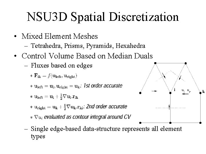
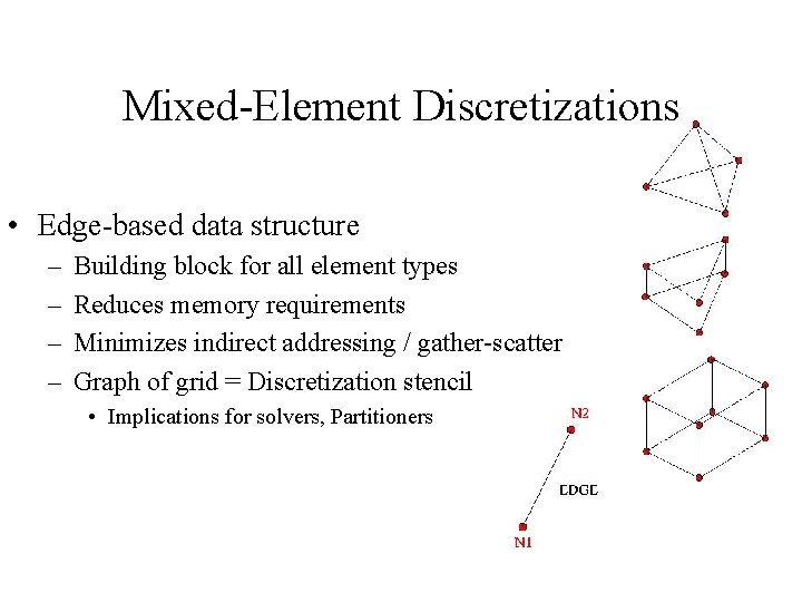
NSU 3 D Spatial Discretization • Mixed Element Meshes – Tetrahedra, Prisms, Pyramids, Hexahedra • Control Volume Based on Median Duals – Fluxes based on edges – Single edge-based data-structure represents all element types

Mixed-Element Discretizations • Edge-based data structure – – Building block for all element types Reduces memory requirements Minimizes indirect addressing / gather-scatter Graph of grid = Discretization stencil • Implications for solvers, Partitioners

NSU 3 D Convergence Acceleration Methods for Steady-State (and Unsteady) Problems • Multigrid Methods – Fully automated agglomeration techniques – Provides convergence rates independent of grid size (usually < 500 MG Cycles) • Implicit Line Solver – Used on each MG Level – Reduces stiffness due to grid anisotropy in Blayer • No Wall Fctns

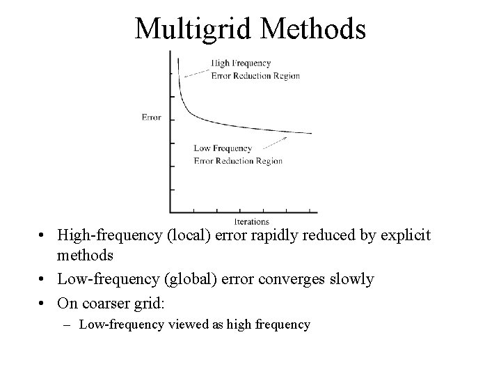
Multigrid Methods • High-frequency (local) error rapidly reduced by explicit methods • Low-frequency (global) error converges slowly • On coarser grid: – Low-frequency viewed as high frequency

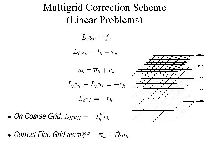
Multigrid Correction Scheme (Linear Problems)

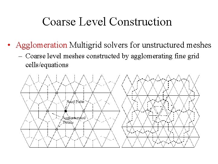
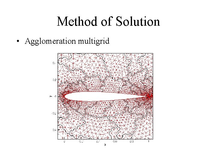
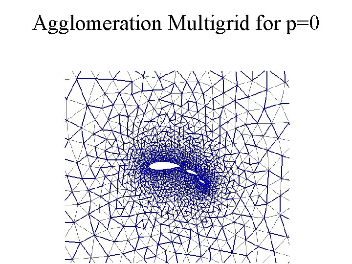
Coarse Level Construction • Agglomeration Multigrid solvers for unstructured meshes – Coarse level meshes constructed by agglomerating fine grid cells/equations

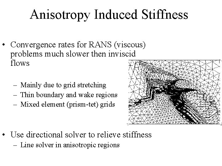
Anisotropy Induced Stiffness • Convergence rates for RANS (viscous) problems much slower then inviscid flows – Mainly due to grid stretching – Thin boundary and wake regions – Mixed element (prism-tet) grids • Use directional solver to relieve stiffness – Line solver in anisotropic regions

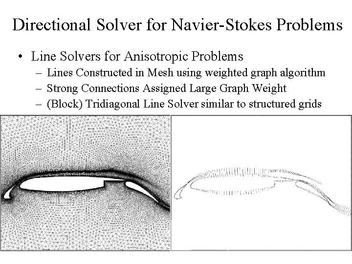
Directional Solver for Navier-Stokes Problems • Line Solvers for Anisotropic Problems – Lines Constructed in Mesh using weighted graph algorithm – Strong Connections Assigned Large Graph Weight – (Block) Tridiagonal Line Solver similar to structured grids

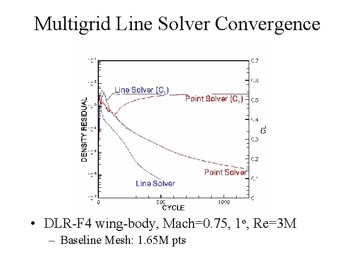
Multigrid Line Solver Convergence • DLR-F 4 wing-body, Mach=0. 75, 1 o, Re=3 M – Baseline Mesh: 1. 65 M pts

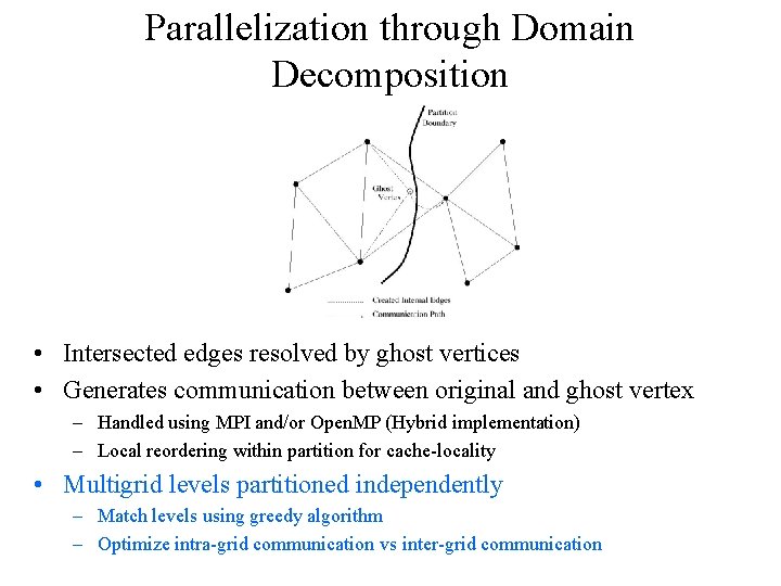
Parallelization through Domain Decomposition • Intersected edges resolved by ghost vertices • Generates communication between original and ghost vertex – Handled using MPI and/or Open. MP (Hybrid implementation) – Local reordering within partition for cache-locality • Multigrid levels partitioned independently – Match levels using greedy algorithm – Optimize intra-grid communication vs inter-grid communication

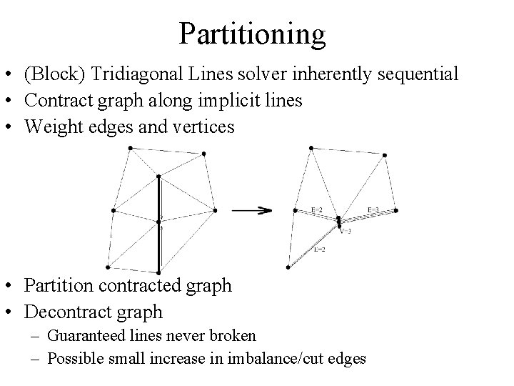
Partitioning • (Block) Tridiagonal Lines solver inherently sequential • Contract graph along implicit lines • Weight edges and vertices • Partition contracted graph • Decontract graph – Guaranteed lines never broken – Possible small increase in imbalance/cut edges

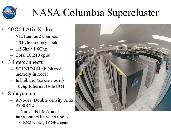
NASA Columbia Supercluster • 20 SGI Atix Nodes – – 512 Itanium 2 cpus each 1 Tbyte memory each 1. 5 Ghz / 1. 6 Ghz Total 10, 240 cpus • 3 Interconnects – SGI NUMAlink (shared memory in node) – Infiniband (across nodes) – 10 Gig Ethernet (File I/O) • Subsystems: – 8 Nodes: Double density Altix 3700 BX 2 – 4 Nodes: NUMAlink 4 interconnect between nodes • BX 2 Nodes, 1. 6 GHz cpus

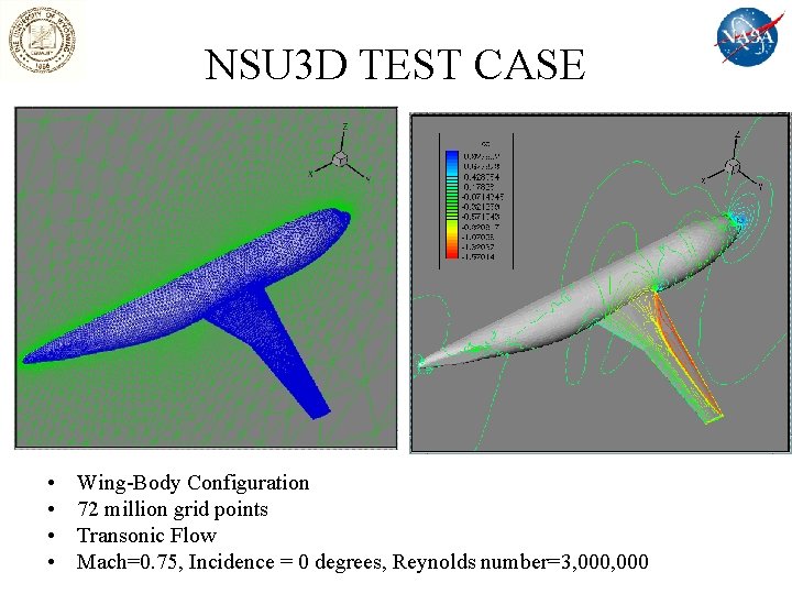
NSU 3 D TEST CASE • • Wing-Body Configuration 72 million grid points Transonic Flow Mach=0. 75, Incidence = 0 degrees, Reynolds number=3, 000

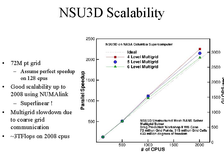
NSU 3 D Scalability • 72 M pt grid – Assume perfect speedup on 128 cpus • Good scalability up to 2008 using NUMAlink – Superlinear ! • Multigrid slowdown due to coarse grid communication • ~3 TFlops on 2008 cpus

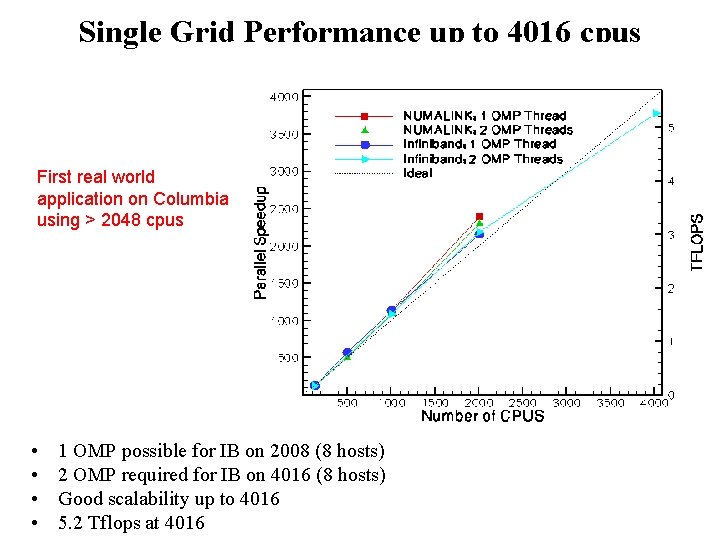
Single Grid Performance up to 4016 cpus First real world application on Columbia using > 2048 cpus • • 1 OMP possible for IB on 2008 (8 hosts) 2 OMP required for IB on 4016 (8 hosts) Good scalability up to 4016 5. 2 Tflops at 4016

Unstructured NS Solver/NASA Columbia Supercomputer • ~100 M pt solutions in 15 minutes • 109 pt solutions can become routine – Ease other bottlenecks (I/O for 109 pts = 400 GB) • High resolution MDO • High resolution Aeroelasticity

Enabling Techniques • Design Optimization – Robust Mesh Deformation (Linear elasticity) – Discrete Adjoint for Flow equations – Discrete Adjoint for Mesh Motion Equations • Mesh sensitivites (Park and Nielsen) – Line-Implicit Agglomeration Multigrid Solver • Flow, flow adjoint, mesh motion, mesh adjoint – Duality preserving formulation • Adjoint discretization requires almost no additional memory over first order-Jacobian used for implicit solver • Modular (subroutine) construction for adjoint and mesh sensitivities – d. R/dx = dr/d(edge)/dx • Similar convegence rates for tangent and adjoint problems

Enabling Techniques • Aeroelasticity – Robust Mesh Deformation (Linear elasticity) – Line-Implicit Agglomeration Multigrid Solver • Flow (implicit time step), mesh motion • Linear multigrid formulation – High-order temporal discretization • Backwards Difference (up to 3 rd order) • Implicit Runge-Kutta (up to fourth order) • Formulation of Geometric Conservation Law for highorder time-stepping – Necessary for non-linear stability

Mesh Motion • Developed for MDO and Aeroelasticity Problems • Emphasis on Robustness – Spring Analogy – Truss Analogy, Beam Analogy – Linear Elasticity: Variable Modulus • Emphasis on Efficiency – Edge based formulation – Gauss Seidel Line Solver with Agglomeration Multigrid – Fully integrated into flow solver

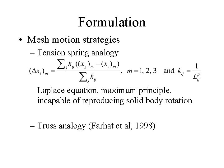
Formulation • Mesh motion strategies – Tension spring analogy Laplace equation, maximum principle, incapable of reproducing solid body rotation – Truss analogy (Farhat et al, 1998)

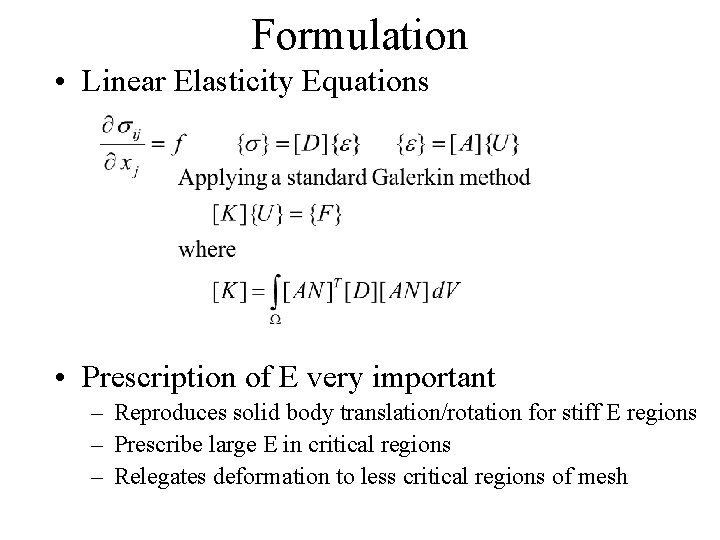
Formulation • Linear Elasticity Equations • Prescription of E very important – Reproduces solid body translation/rotation for stiff E regions – Prescribe large E in critical regions – Relegates deformation to less critical regions of mesh

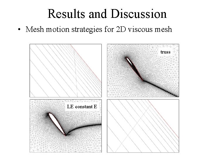
Results and Discussion • Mesh motion strategies for 2 D viscous mesh spring LE constant E truss LE variable E

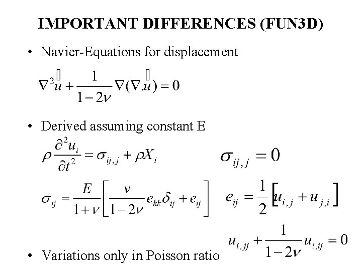
IMPORTANT DIFFERENCES (FUN 3 D) • Navier-Equations for displacement • Derived assuming constant E • Variations only in Poisson ratio

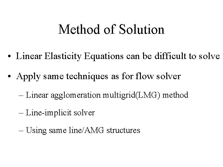
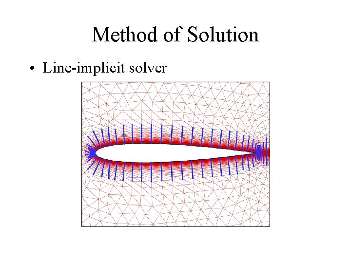
Method of Solution • Linear Elasticity Equations can be difficult to solve • Apply same techniques as for flow solver – Linear agglomeration multigrid(LMG) method – Line-implicit solver – Using same line/AMG structures

Method of Solution • Agglomeration multigrid

Method of Solution • Line-implicit solver Strong coupling

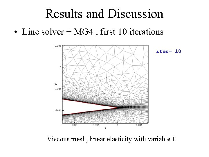
Results and Discussion • Line solver + MG 4 , first 10 iterations iter= 10 0 1 2 3 4 5 6 7 8 9 Viscous mesh, linear elasticity with variable E

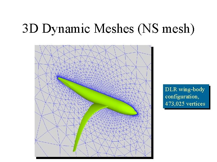
3 D Dynamic Meshes (NS mesh) DLR wing-body configuration, 473, 025 vertices

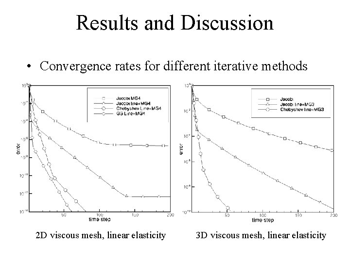
Results and Discussion • Convergence rates for different iterative methods 2 D viscous mesh, linear elasticity 3 D viscous mesh, linear elasticity

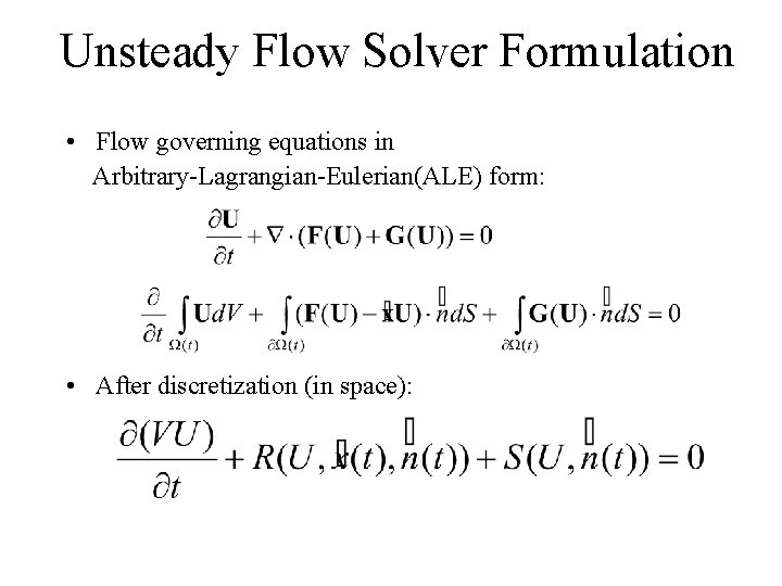
Unsteady Flow Solver Formulation • Flow governing equations in Arbitrary-Lagrangian-Eulerian(ALE) form: • After discretization (in space):

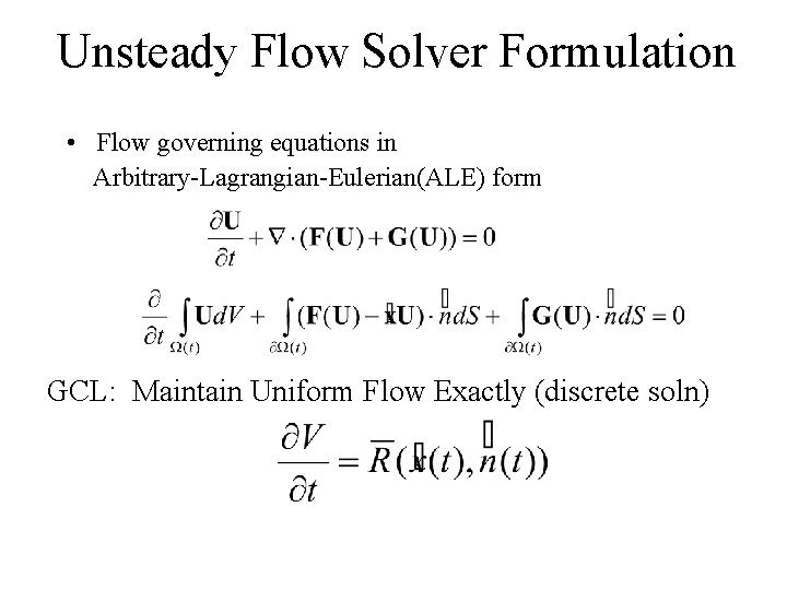
Unsteady Flow Solver Formulation • Flow governing equations in Arbitrary-Lagrangian-Eulerian(ALE) form GCL: Maintain Uniform Flow Exactly (discrete soln)

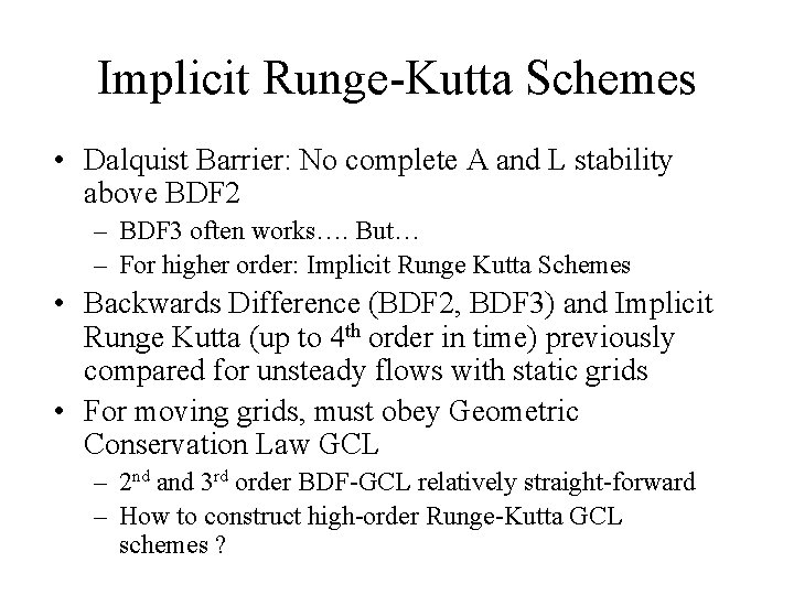
Implicit Runge-Kutta Schemes • Dalquist Barrier: No complete A and L stability above BDF 2 – BDF 3 often works…. But… – For higher order: Implicit Runge Kutta Schemes • Backwards Difference (BDF 2, BDF 3) and Implicit Runge Kutta (up to 4 th order in time) previously compared for unsteady flows with static grids • For moving grids, must obey Geometric Conservation Law GCL – 2 nd and 3 rd order BDF-GCL relatively straight-forward – How to construct high-order Runge-Kutta GCL schemes ?

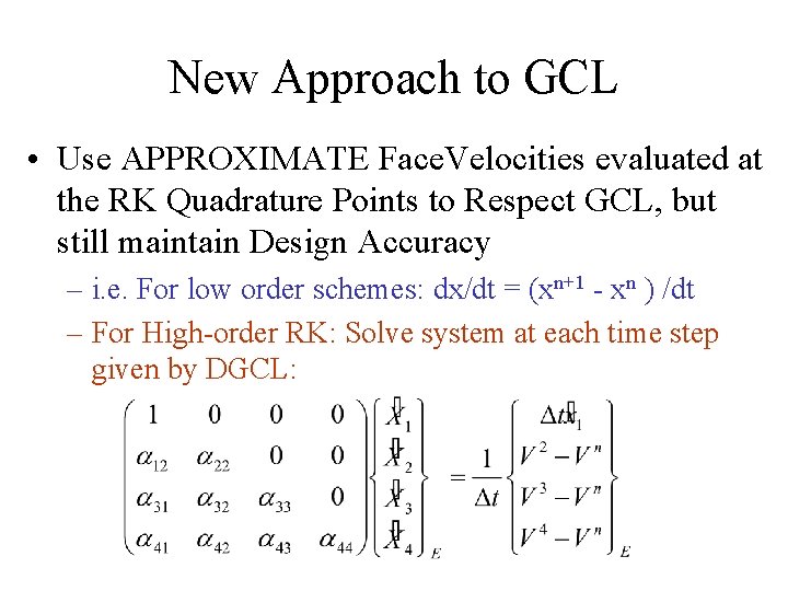
New Approach to GCL • Use APPROXIMATE Face. Velocities evaluated at the RK Quadrature Points to Respect GCL, but still maintain Design Accuracy – i. e. For low order schemes: dx/dt = (xn+1 - xn ) /dt – For High-order RK: Solve system at each time step given by DGCL:

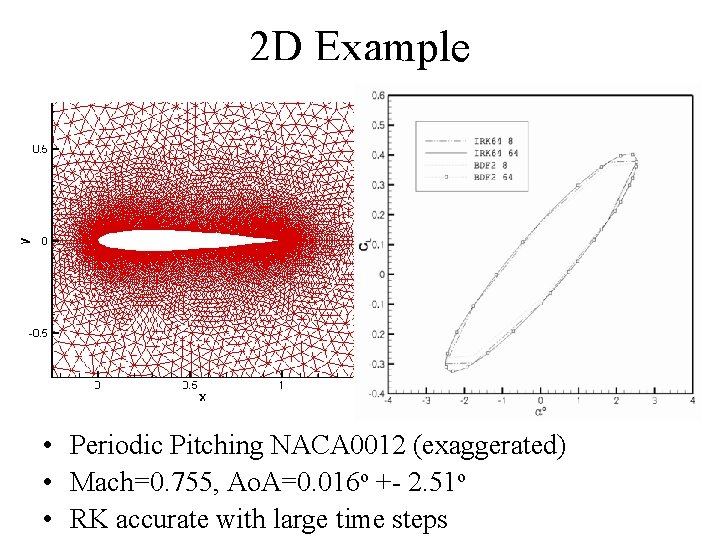
2 D Example • Periodic Pitching NACA 0012 (exaggerated) • Mach=0. 755, Ao. A=0. 016 o +- 2. 51 o • RK accurate with large time steps

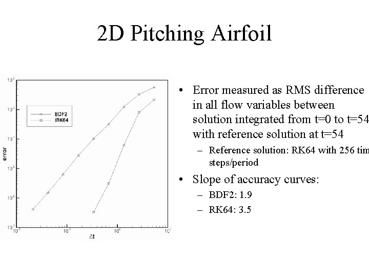
2 D Pitching Airfoil • Error measured as RMS difference in all flow variables between solution integrated from t=0 to t=54 with reference solution at t=54 – Reference solution: RK 64 with 256 tim steps/period • Slope of accuracy curves: – BDF 2: 1. 9 – RK 64: 3. 5

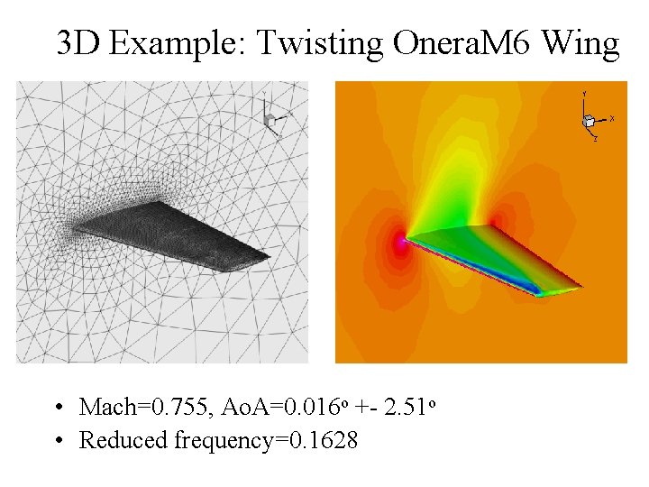
3 D Example: Twisting Onera. M 6 Wing • Mach=0. 755, Ao. A=0. 016 o +- 2. 51 o • Reduced frequency=0. 1628

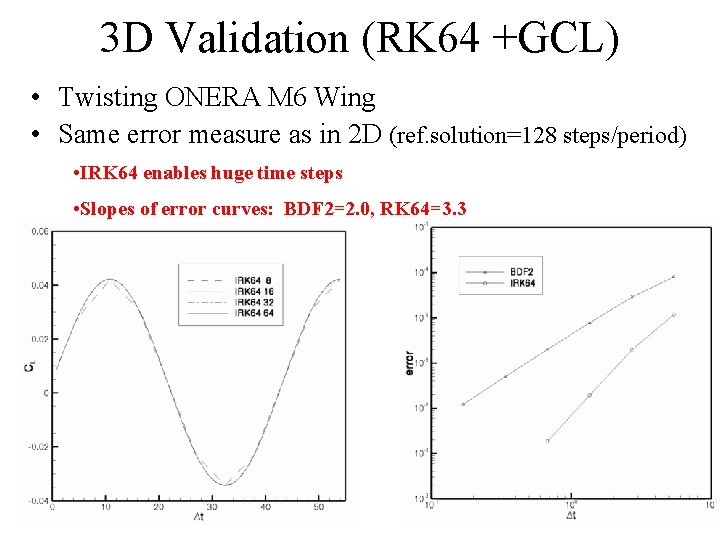
3 D Validation (RK 64 +GCL) • Twisting ONERA M 6 Wing • Same error measure as in 2 D (ref. solution=128 steps/period) • IRK 64 enables huge time steps • Slopes of error curves: BDF 2=2. 0, RK 64=3. 3

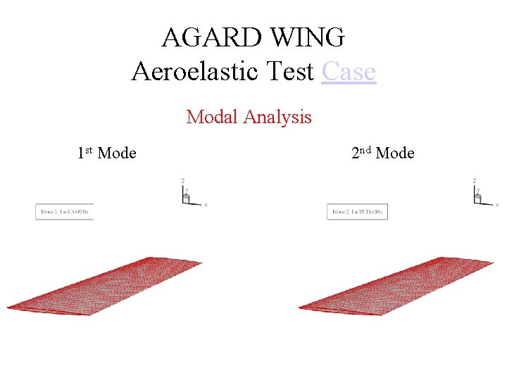
AGARD WING Aeroelastic Test Case Modal Analysis 1 st Mode 2 nd Mode

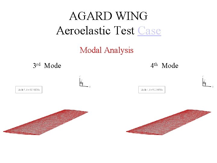
AGARD WING Aeroelastic Test Case Modal Analysis 3 rd Mode 4 th Mode

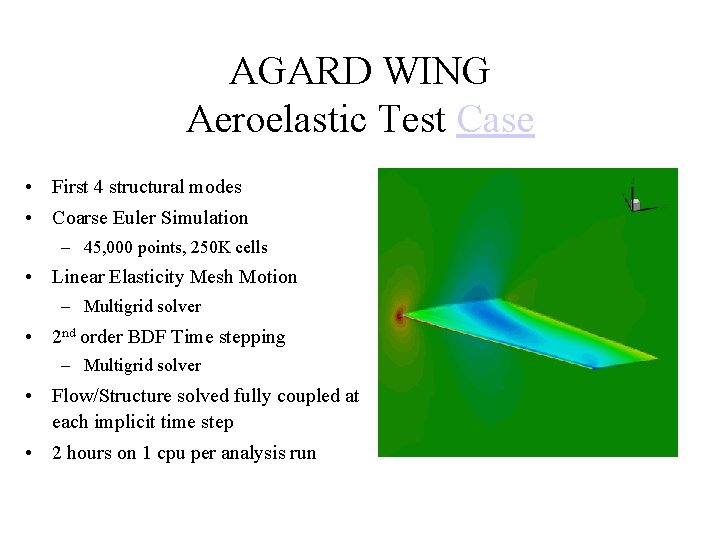
AGARD WING Aeroelastic Test Case • First 4 structural modes • Coarse Euler Simulation – 45, 000 points, 250 K cells • Linear Elasticity Mesh Motion – Multigrid solver • 2 nd order BDF Time stepping – Multigrid solver • Flow/Structure solved fully coupled at each implicit time step • 2 hours on 1 cpu per analysis run

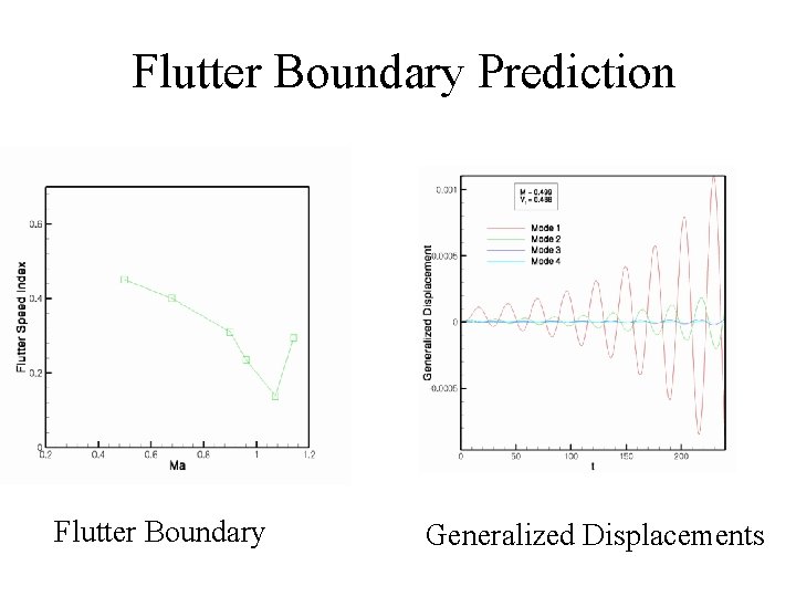
Flutter Boundary Prediction Flutter Boundary Generalized Displacements

Current and Future Work • Investigate benefits of Implicit Runge-Kutta – 4 th order temporal accuracy • Investigate optimal time-step size and convergence criteria • Develop automated temporal-error control scheme • Viscous simulations, Finer Meshes – 5 M pt Unsteady Navier-Stokes solutions : • 2 -4 hours on 128 cpus of Columbia • Adjoint for unsteady problems – Time domain – Frequency domain

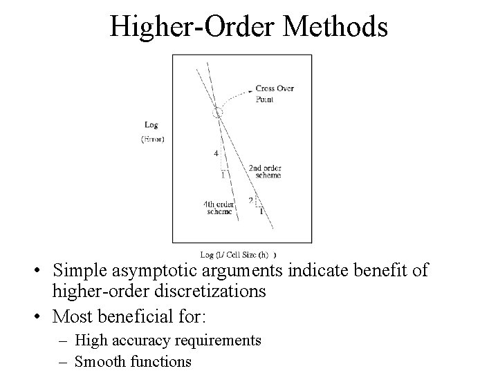
Higher-Order Methods • Simple asymptotic arguments indicate benefit of higher-order discretizations • Most beneficial for: – High accuracy requirements – Smooth functions

Motivation • Higher-order methods successes – Acoustics – Large Eddy Simulation (structured grids) – Other areas • High-order methods not demonstrated in: – – Aerodynamics, Hydrodynamics Unstructured mesh LES Industrial CFD Cost effectiveness not demonstrated: • Cost of discretization • Efficient solution of complex discrete equations

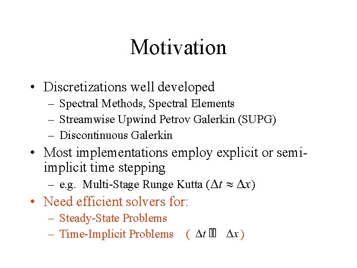
Motivation • Discretizations well developed – Spectral Methods, Spectral Elements – Streamwise Upwind Petrov Galerkin (SUPG) – Discontinuous Galerkin • Most implementations employ explicit or semiimplicit time stepping – e. g. Multi-Stage Runge Kutta ( ) • Need efficient solvers for: – Steady-State Problems – Time-Implicit Problems ( )

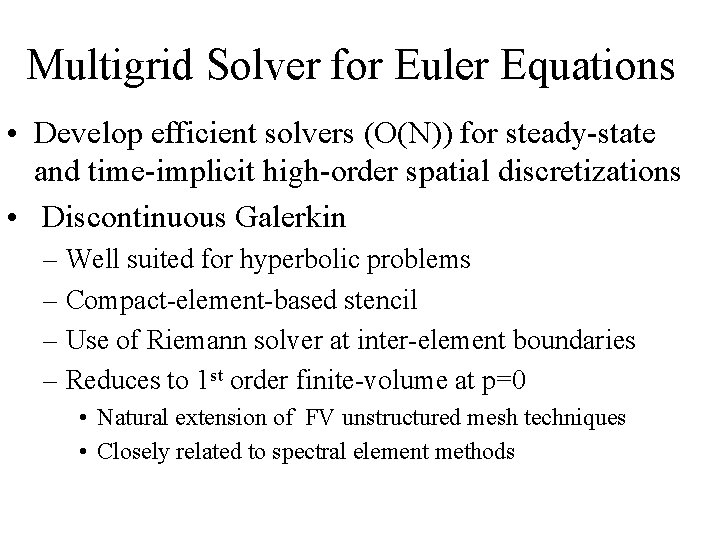
Multigrid Solver for Euler Equations • Develop efficient solvers (O(N)) for steady-state and time-implicit high-order spatial discretizations • Discontinuous Galerkin – Well suited for hyperbolic problems – Compact-element-based stencil – Use of Riemann solver at inter-element boundaries – Reduces to 1 st order finite-volume at p=0 • Natural extension of FV unstructured mesh techniques • Closely related to spectral element methods

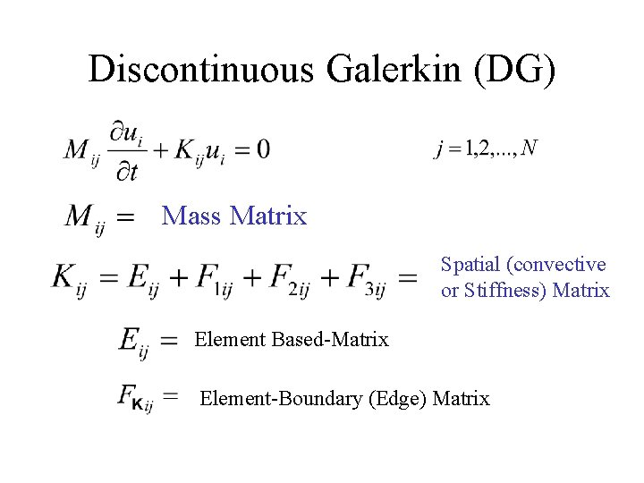
Discontinuous Galerkin (DG) Mass Matrix Spatial (convective or Stiffness) Matrix Element Based-Matrix Element-Boundary (Edge) Matrix

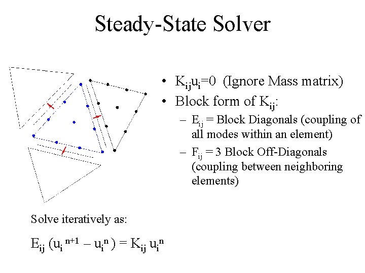
Steady-State Solver • Kijui=0 (Ignore Mass matrix) • Block form of Kij: – Eij = Block Diagonals (coupling of all modes within an element) – Fij = 3 Block Off-Diagonals (coupling between neighboring elements) Solve iteratively as: Eij (ui n+1 – uin ) = Kij uin

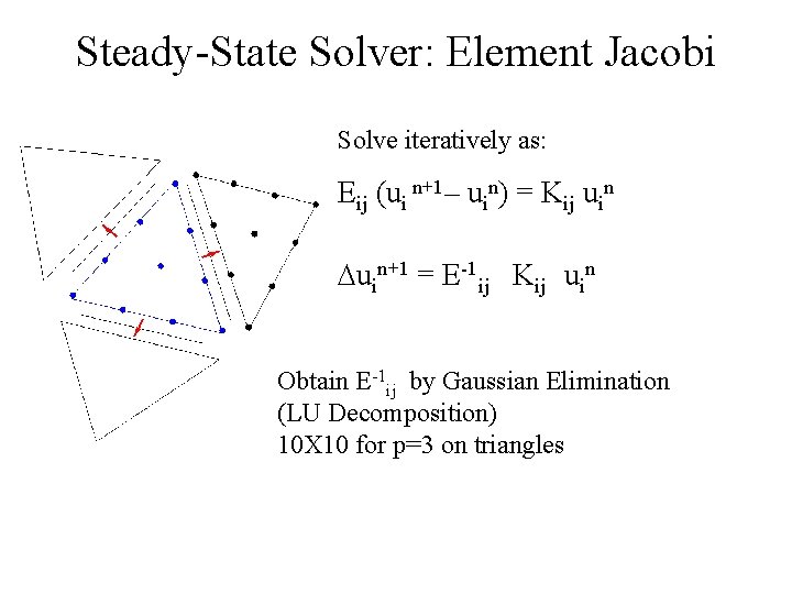
Steady-State Solver: Element Jacobi Solve iteratively as: Eij (ui n+1– uin) = Kij uin Duin+1 = E-1 ij Kij uin Obtain E-1 ij by Gaussian Elimination (LU Decomposition) 10 X 10 for p=3 on triangles

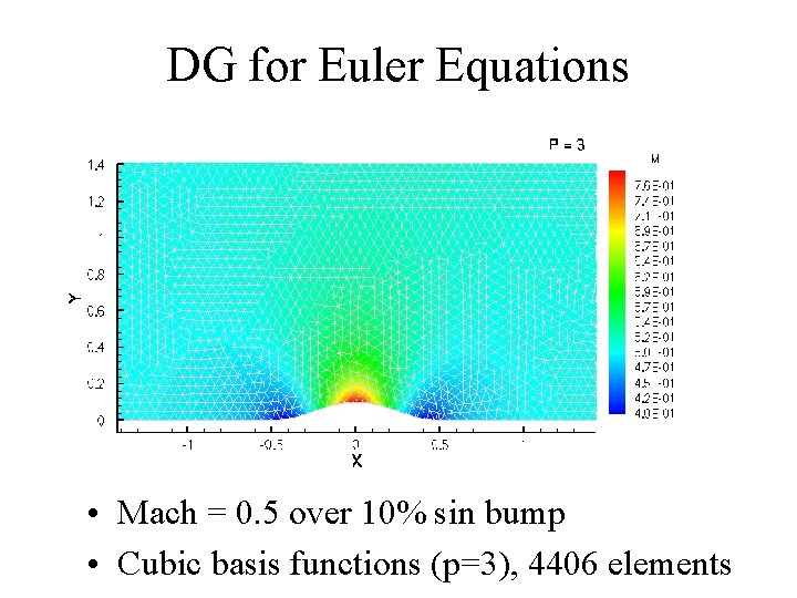
DG for Euler Equations • Mach = 0. 5 over 10% sin bump • Cubic basis functions (p=3), 4406 elements

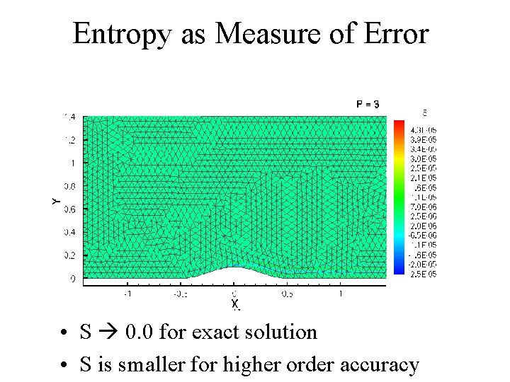
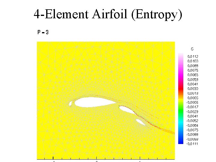
Entropy as Measure of Error • S 0. 0 for exact solution • S is smaller for higher order accuracy

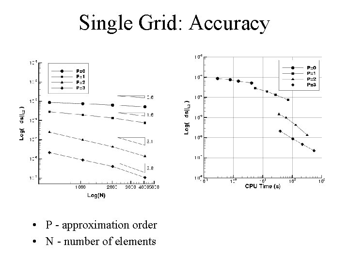
Single Grid: Accuracy • P - approximation order • N - number of elements

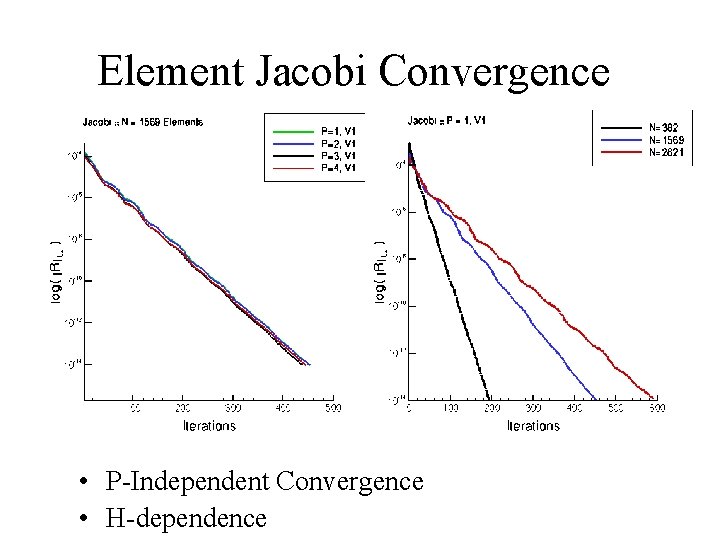
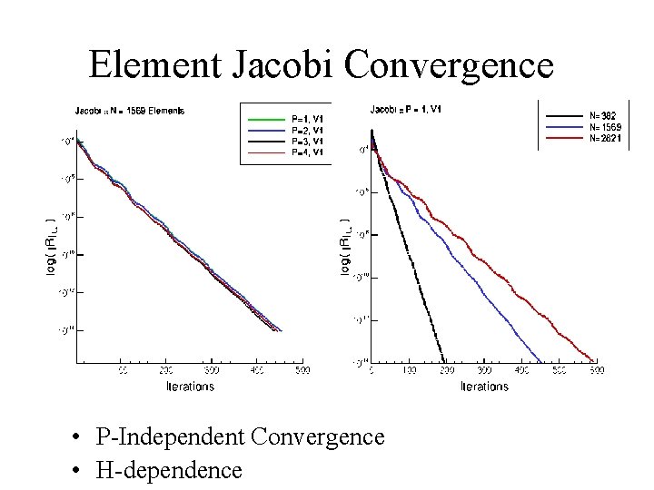
Element Jacobi Convergence • P-Independent Convergence • H-dependence

Improving Convergence -Dependence H • Requires implicitness between grid elements • Multigrid methods based on use of coarser meshes for accelerating solution on fine mesh

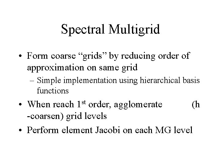
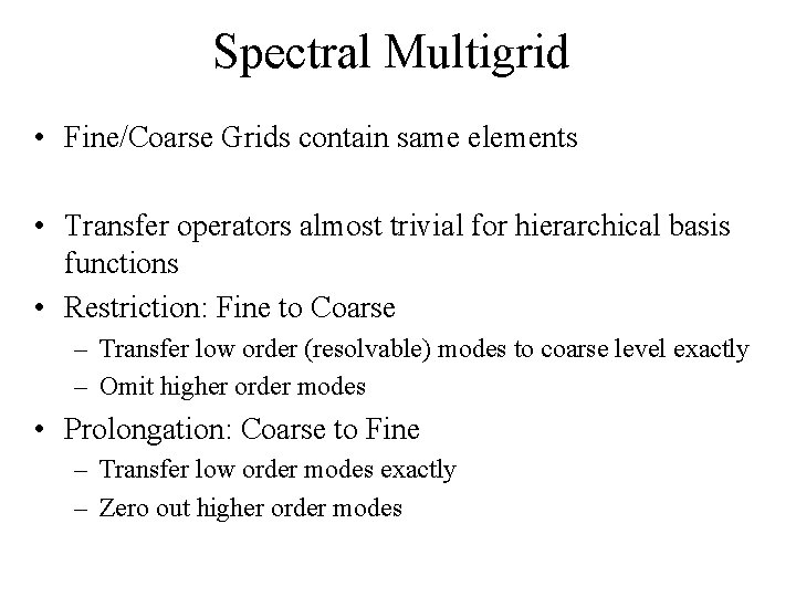
Spectral Multigrid • Form coarse “grids” by reducing order of approximation on same grid – Simplementation using hierarchical basis functions • When reach 1 st order, agglomerate (h -coarsen) grid levels • Perform element Jacobi on each MG level

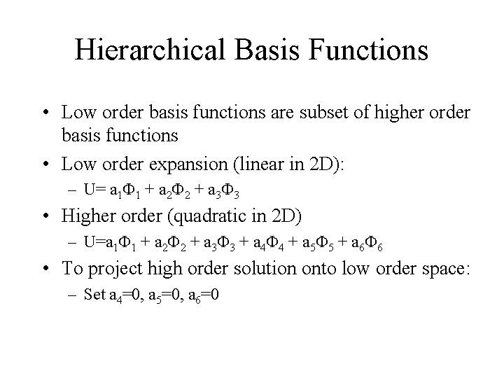
Hierarchical Basis Functions • Low order basis functions are subset of higher order basis functions • Low order expansion (linear in 2 D): – U= a 1 F 1 + a 2 F 2 + a 3 F 3 • Higher order (quadratic in 2 D) – U=a 1 F 1 + a 2 F 2 + a 3 F 3 + a 4 F 4 + a 5 F 5 + a 6 F 6 • To project high order solution onto low order space: – Set a 4=0, a 5=0, a 6=0

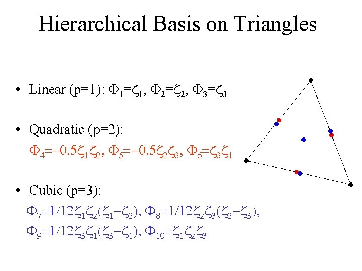
Hierarchical Basis on Triangles • Linear (p=1): F 1=z 1, F 2=z 2, F 3=z 3 • Quadratic (p=2): F 4=-0. 5 z 1 z 2, F 5=-0. 5 z 2 z 3, F 6=z 3 z 1 • Cubic (p=3): F 7=1/12 z 1 z 2(z 1 -z 2), F 8=1/12 z 2 z 3(z 2 -z 3), F 9=1/12 z 3 z 1(z 3 -z 1), F 10=z 1 z 2 z 3

Spectral Multigrid • Fine/Coarse Grids contain same elements • Transfer operators almost trivial for hierarchical basis functions • Restriction: Fine to Coarse – Transfer low order (resolvable) modes to coarse level exactly – Omit higher order modes • Prolongation: Coarse to Fine – Transfer low order modes exactly – Zero out higher order modes

Element Jacobi Convergence • P-Independent Convergence • H-dependence

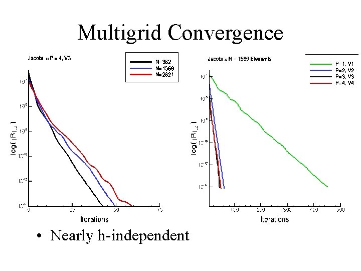
Multigrid Convergence • Nearly h-independent

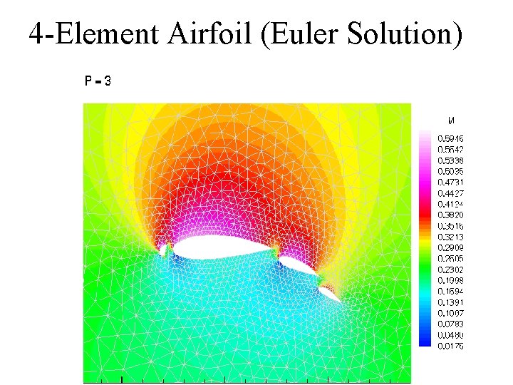
4 -Element Airfoil (Euler Solution)

4 -Element Airfoil (Entropy)

Agglomeration Multigrid for p=0

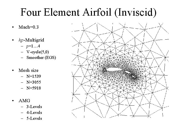
Four Element Airfoil (Inviscid) • Mach=0. 3 • hp-Multigrid – p=1… 4 – V-cycle(5, 0) – Smoother (EGS) • Mesh size – N=1539 – N=3055 – N=5918 • AMG – 3 -Levels – 4 -Levels – 5 -Levels

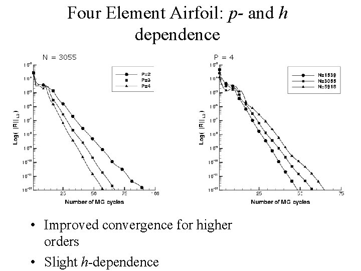
Four Element Airfoil: p- and h dependence N = 3055 P=4 • Improved convergence for higher orders • Slight h-dependence

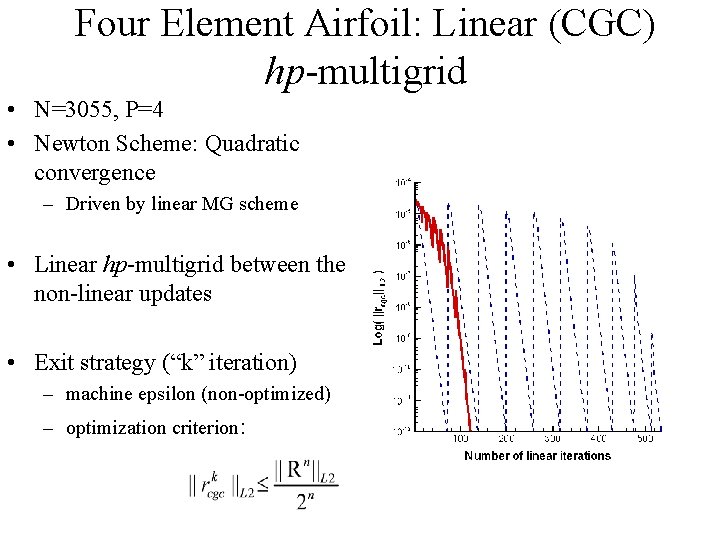
Four Element Airfoil: Linear (CGC) hp-multigrid • N=3055, P=4 • Newton Scheme: Quadratic convergence – Driven by linear MG scheme • Linear hp-multigrid between the non-linear updates • Exit strategy (“k” iteration) – machine epsilon (non-optimized) – optimization criterion:

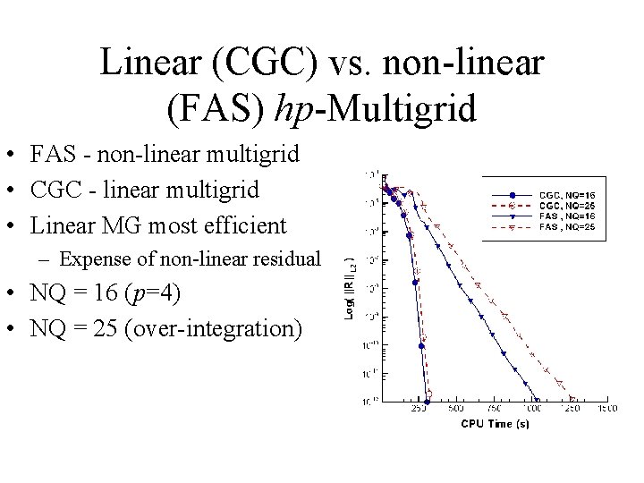
Linear (CGC) vs. non-linear (FAS) hp-Multigrid • FAS - non-linear multigrid • CGC - linear multigrid • Linear MG most efficient – Expense of non-linear residual • NQ = 16 (p=4) • NQ = 25 (over-integration)

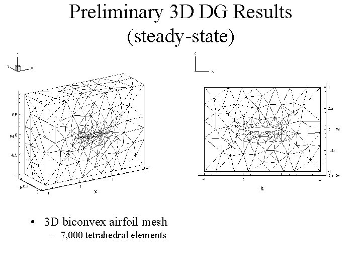
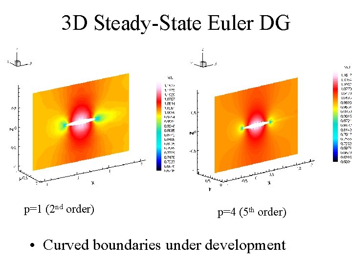
Preliminary 3 D DG Results (steady-state) • 3 D biconvex airfoil mesh – 7, 000 tetrahedral elements

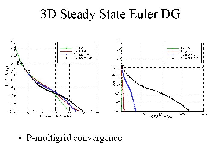
3 D Steady State Euler DG • P-multigrid convergence

3 D Steady-State Euler DG p=1 (2 nd order) p=4 (5 th order) • Curved boundaries under development

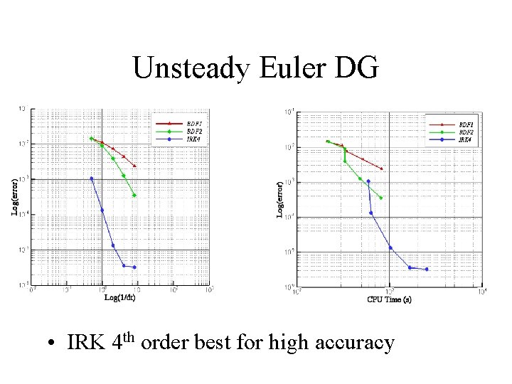
Unsteady DG (2 D) • Implicit time-stepping for low reduced frequency problems and small explicit time step restriction of high -order schemes • Balance Temporal/Spatial Discretization Errors – p=3(4 th order in space) – BDF 1, BDF 2, IRK 4 • Runge-Kutta is equivalent to DG in time • Use h-p multigrid to solve non-linear problem at each implicit time step

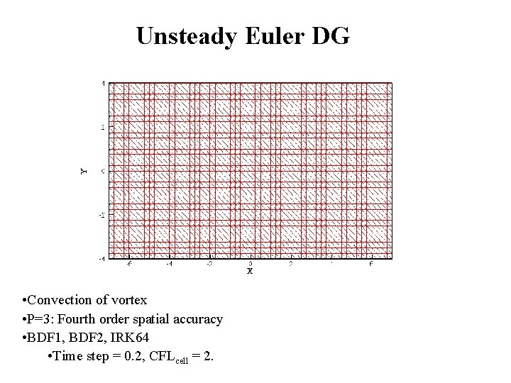
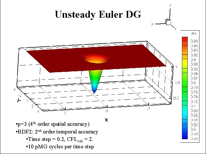
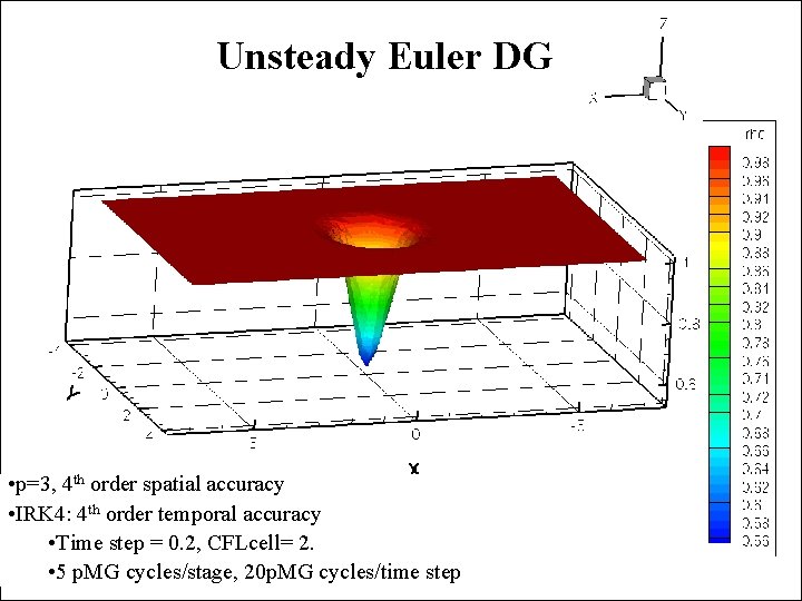
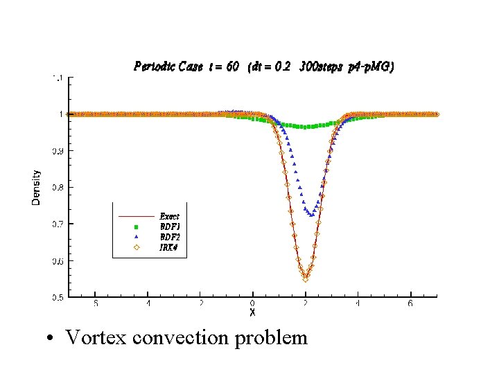
Unsteady Euler DG • Convection of vortex • P=3: Fourth order spatial accuracy • BDF 1, BDF 2, IRK 64 • Time step = 0. 2, CFLcell = 2.

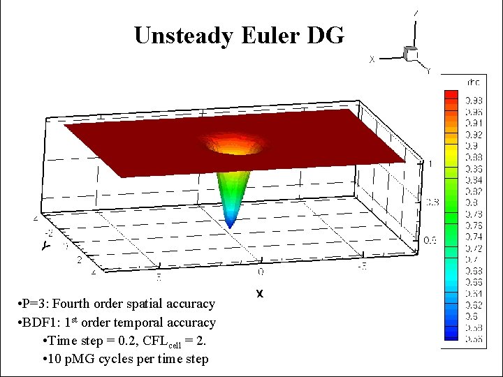
Unsteady Euler DG • P=3: Fourth order spatial accuracy • BDF 1: 1 st order temporal accuracy • Time step = 0. 2, CFLcell = 2. • 10 p. MG cycles per time step

Unsteady Euler DG • p=3 (4 th order spatial accuracy) • BDF 2: 2 nd order temporal accuracy • Time step = 0. 2, CFLcell = 2. • 10 p. MG cycles per time step

Unsteady Euler DG • p=3, 4 th order spatial accuracy • IRK 4: 4 th order temporal accuracy • Time step = 0. 2, CFLcell= 2. • 5 p. MG cycles/stage, 20 p. MG cycles/time step

Unsteady Euler DG • Vortex convection problem

Unsteady Euler DG • IRK 4 th order best for high accuracy

Future Work • Higher order schemes still costly in terms of cpu time compared to 2 nd order schemes – Will these become viable for industrial calculations? • H-P Adaptivity – Flexible approach to use higher order where beneficial – Incorporate hp-Multigrid with hp Adaptivity • Extend to: – 3 D Viscous – Unsteady – Dynamic Meshes