Programming with Matlab Day 2 More about Loops

Programming with Matlab Day 2: More about Loops, Vectors and Matrices

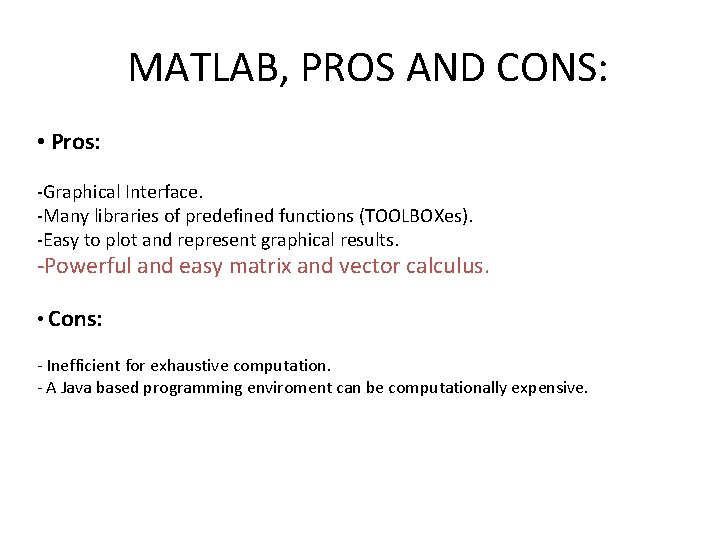
MATLAB, PROS AND CONS: • Pros: -Graphical Interface. -Many libraries of predefined functions (TOOLBOXes). -Easy to plot and represent graphical results. -Powerful and easy matrix and vector calculus. • Cons: - Inefficient for exhaustive computation. - A Java based programming enviroment can be computationally expensive.

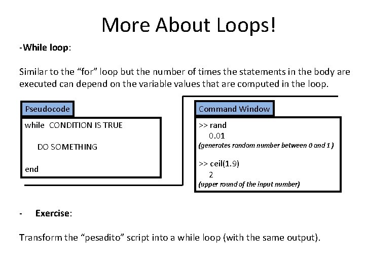
More About Loops! -While loop: Similar to the “for” loop but the number of times the statements in the body are executed can depend on the variable values that are computed in the loop. Pseudocode Command Window while CONDITION IS TRUE >> rand 0. 01 DO SOMETHING end (generates random number between 0 and 1 ) >> ceil(1. 9) 2 (upper round of the input number) - Exercise: Transform the “pesadito” script into a while loop (with the same output).

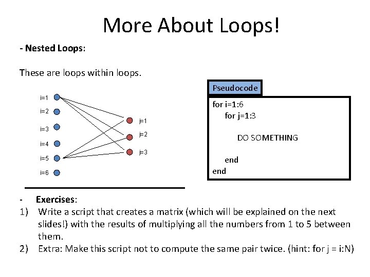
More About Loops! - Nested Loops: These are loops within loops. Pseudocode i=1 i=2 j=1 i=3 j=2 i=4 i=5 i=6 j=3 for i=1: 6 for j=1: 3 DO SOMETHING end - Exercises: 1) Write a script that creates a matrix (which will be explained on the next slides!) with the results of multiplying all the numbers from 1 to 5 between them. 2) Extra: Make this script not to compute the same pair twice. (hint: for j = i: N)

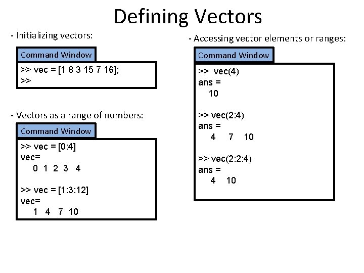
- Initializing vectors: Defining Vectors - Accessing vector elements or ranges: Command Window >> vec = [1 8 3 15 7 16]; >> >> vec(4) ans = 10 - Vectors as a range of numbers: Command Window >> vec = [0: 4] vec= 0 1 2 3 4 >> vec = [1: 3: 12] vec= 1 4 7 10 >> vec(2: 4) ans = 4 7 10 >> vec(2: 2: 4) ans = 4 10

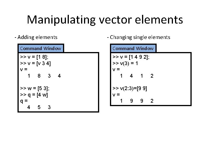
Manipulating vector elements - Adding elements - Changing single elements Command Window >> v = [1 8]; >> v = [v 3 4] v= 1 8 3 >> v = [1 4 9 2]; >> v(3) = 1 v= 1 4 1 2 >> w = [5 3]; >> q = [4 w] q= 4 5 3 4 >> v(2: 3)=[9 9] v= 1 9 9 2

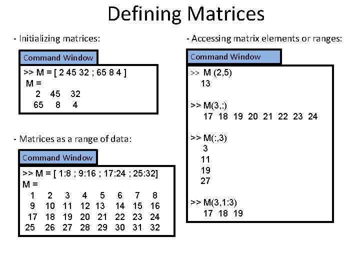
Defining Matrices - Initializing matrices: - Accessing matrix elements or ranges: Command Window >> M = [ 2 45 32 ; 65 8 4 ] M= 2 45 32 65 8 4 >> M (2, 5) 13 - Matrices as a range of data: >> M(: , 3) 3 11 19 27 Command Window >> M = [ 1: 8 ; 9: 16 ; 17: 24 ; 25: 32] M= 1 2 3 4 5 6 7 8 9 10 11 12 13 14 15 16 17 18 19 20 21 22 23 24 25 26 27 28 29 30 31 32 >> M(3, : ) 17 18 19 20 21 22 23 24 >> M(3, 1: 3) 17 18 19

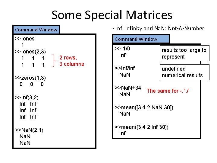
Some Special Matrices - Inf: Infinity and Na. N: Not-A-Number Command Window >> ones 1 >> ones(2, 3) 1 1 1 >>zeros(1, 3) 0 0 0 >>Inf(3, 2) Inf Inf Inf >>Na. N(2, 1) Na. N Command Window 2 rows, 3 columns >> 1/0 Inf results too large to represent >>Inf/Inf Na. N undefined numerical results >>Na. N+34 The same for -, *, / Na. N >>mean([3 4 2 Na. N 30]) Na. N >>mean([3 4 2 Inf 30]) Inf

Operating with vectors and matrices - Basic operations (element-by-element): Command Window >> v=[1: 4] v= 1 2 3 4 >> v*5 5 10 15 20 >> v-3 -2 -1 0 1 >> v / 6; >> v * 5. 5; Scalar operations are performed element by element. Command Window >> M = [1 2 ; 3 4 ] >> N = [2. 5 3 ; 2 1] M= 1 2 3 4 N= 2. 5 2. 0 3. 0 1. 0 >> M+N 3. 5 5. 0 >> M. *N 2. 5 6. 0 4. 0 >> M. /N; >> M. ^2; The dot indicates an element-by-element operation

Basic functions - For vectors: - For matrices: Command Window >>v=[4 8 3 2] v= 4 8 3 >> M=[3 6 1 4; 8 0 2 4] M= 3 6 1 4 8 0 2 4 2 >> length(v) 4 >> max(v) 8 >> min(v) 2 >> max(M) 8 6 2 >> sum(v) 17 >> mean(v) 4. 25 >>size(M) 2 4 >>length(M) 4 >> std(v) 2. 63 length of largest dimension 4 >> sum(M) 11 6 3 >> mean(M) 5. 5 3. 0 1. 5 operating along columns 8 4. 0

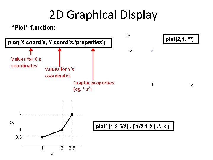
2 D Graphical Display -“Plot” function: plot( X coord´s, Y coord´s, ’properties’) Values for X´s coordinates plot(2, 1, '*') Values for Y´s coordinates Graphic properties (eg. ‘-. r’) plot( [1 2 5/2] , [ 1/2 1 2 ] , ‘. -k')

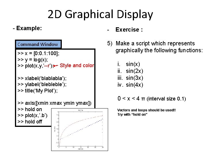
2 D Graphical Display - Example: Command Window >> x = [0: 0. 1: 100]; >> y = log(x); >> plot(x, y, ’--r’); Style and color >> xlabel(‘blablabla’); >> ylabel(‘blebleble’); >> title(‘My Plot’); >> axis([xmin xmax ymin ymax]) >> hold on >> plot(x, ’. b’) >> hold off - Exercise : 5) Make a script which represents graphically the following functions: i. iii. iv. sin(x) sin(2 x) sin(3 x) sin(4 x) 0 < x < 4 π (interval size 0. 1) Vectors and loops should be used!! Try with “hold on”

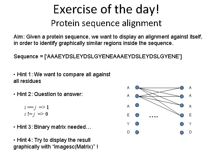
Exercise of the day! Protein sequence alignment Aim: Given a protein sequence, we want to display an alignment against itself, in order to identify graphically similar regions inside the sequence. Sequence = [‘AAAEYDSLEYDSLGYENE’] • Hint 1: We want to compare all against all residues • Hint 2: Question to answer: i == j => 1 i != j => 0 • Hint 3: Binary matrix needed… • Hint 4: Try to display the result graphically with “imagesc(Matrix)” ! A A A E …. E Y Y D D

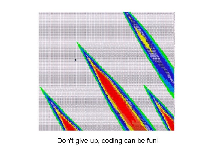
Don’t give up, coding can be fun!