Programming Search How can we control the search

Programming Search How can we control the search in a finite domain programming solver

Overview • • • Finite Domain Search Variable Selection Value Selection Splitting Complex Search Strategies Autonomous Search

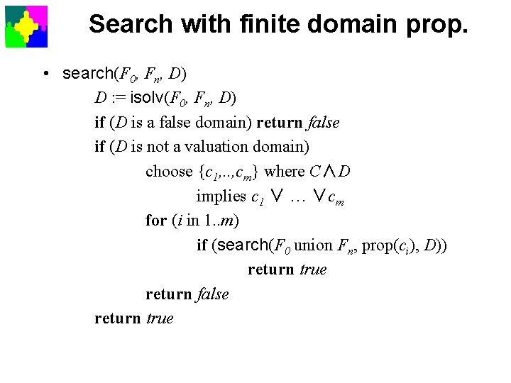
Search with finite domain prop. • search(F 0, Fn, D) D : = isolv(F 0, Fn, D) if (D is a false domain) return false if (D is not a valuation domain) choose {c 1, . . , cm} where C∧D implies c 1 ∨ … ∨cm for (i in 1. . m) if (search(F 0 union Fn, prop(ci), D)) return true return false return true

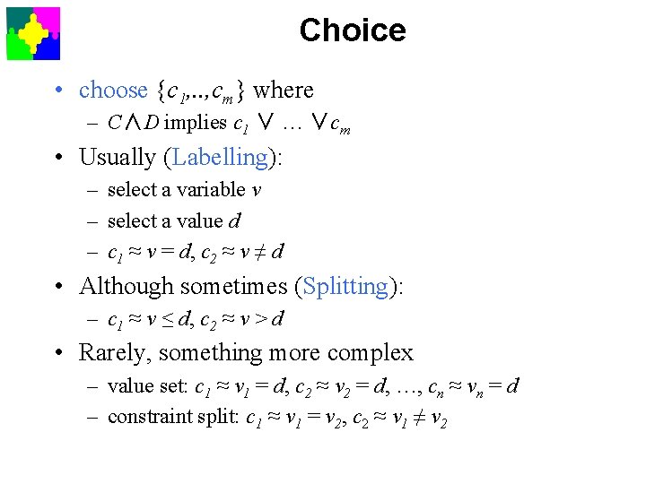
Choice • choose {c 1, . . , cm} where – C∧D implies c 1 ∨ … ∨cm • Usually (Labelling): – select a variable v – select a value d – c 1 ≈ v = d, c 2 ≈ v ≠ d • Although sometimes (Splitting): – c 1 ≈ v ≤ d, c 2 ≈ v > d • Rarely, something more complex – value set: c 1 ≈ v 1 = d, c 2 ≈ v 2 = d, …, cn ≈ vn = d – constraint split: c 1 ≈ v 1 = v 2, c 2 ≈ v 1 ≠ v 2

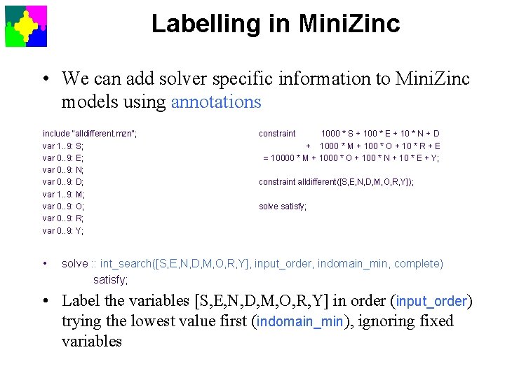
Labelling in Mini. Zinc • We can add solver specific information to Mini. Zinc models using annotations include "alldifferent. mzn"; var 1. . 9: S; var 0. . 9: E; var 0. . 9: N; var 0. . 9: D; var 1. . 9: M; var 0. . 9: O; var 0. . 9: R; var 0. . 9: Y; • constraint 1000 * S + 100 * E + 10 * N + D + 1000 * M + 100 * O + 10 * R + E = 10000 * M + 1000 * O + 100 * N + 10 * E + Y; constraint alldifferent([S, E, N, D, M, O, R, Y]); solve satisfy; solve : : int_search([S, E, N, D, M, O, R, Y], input_order, indomain_min, complete) satisfy; • Label the variables [S, E, N, D, M, O, R, Y] in order (input_order) trying the lowest value first (indomain_min), ignoring fixed variables

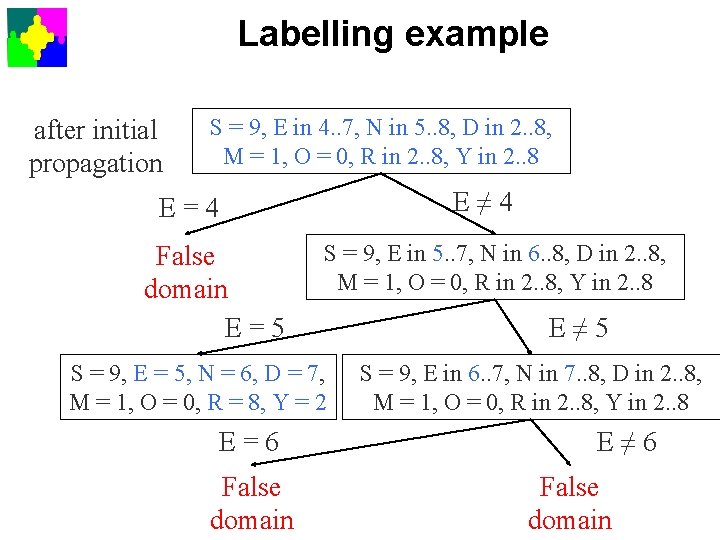
Labelling example after initial propagation S = 9, E in 4. . 7, N in 5. . 8, D in 2. . 8, M = 1, O = 0, R in 2. . 8, Y in 2. . 8 E≠ 4 E=4 False domain E=5 S = 9, E in 5. . 7, N in 6. . 8, D in 2. . 8, M = 1, O = 0, R in 2. . 8, Y in 2. . 8 S = 9, E = 5, N = 6, D = 7, M = 1, O = 0, R = 8, Y = 2 E=6 False domain E≠ 5 S = 9, E in 6. . 7, N in 7. . 8, D in 2. . 8, M = 1, O = 0, R in 2. . 8, Y in 2. . 8 E≠ 6 False domain

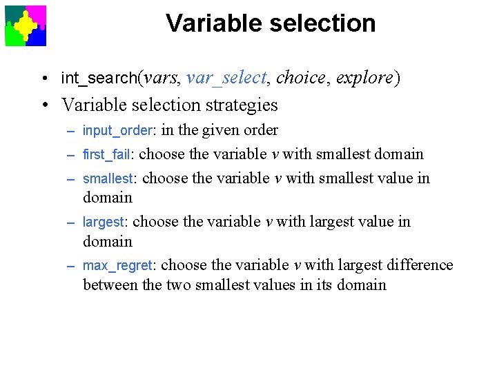
Variable selection • int_search(vars, var_select, choice, explore) • Variable selection strategies – input_order: in the given order – first_fail: choose the variable v with smallest domain – smallest: choose the variable v with smallest value in domain – largest: choose the variable v with largest value in domain – max_regret: choose the variable v with largest difference between the two smallest values in its domain

First Fail Labelling • One useful heuristic is the first-fail principle “To succeed, try first where you are most likely to fail” • At each step choose the variable with the smallest domain. • Do this dynamically based on the domain size after propagation.

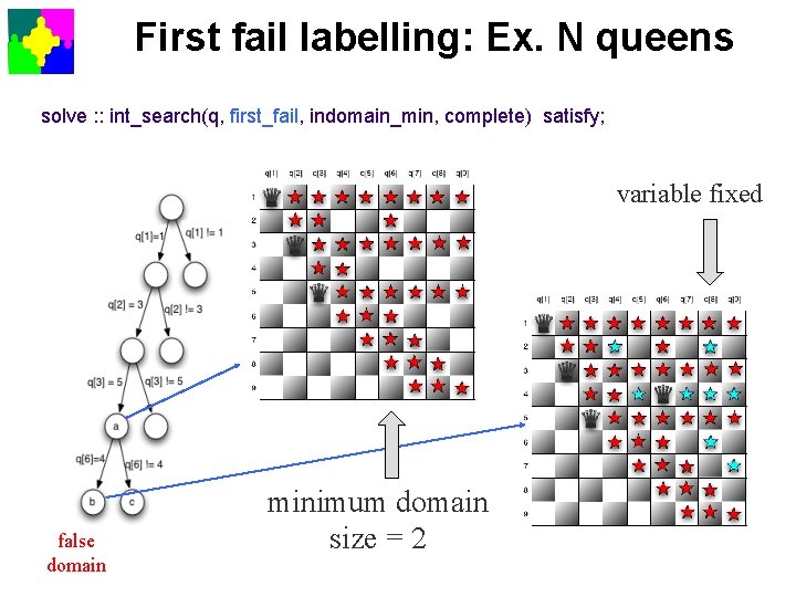
First fail labelling: Ex. N queens solve : : int_search(q, first_fail, indomain_min, complete) satisfy; variable fixed false domain minimum domain size = 2

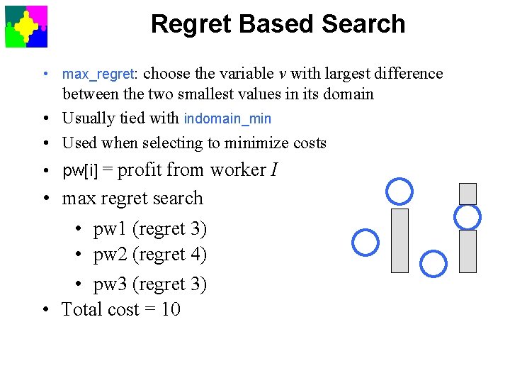
Regret Based Search • max_regret: choose the variable v with largest difference between the two smallest values in its domain • Usually tied with indomain_min • Used when selecting to minimize costs • pw[i] = profit from worker I • max regret search • pw 1 (regret 3) • pw 2 (regret 4) • pw 3 (regret 3) • Total cost = 10

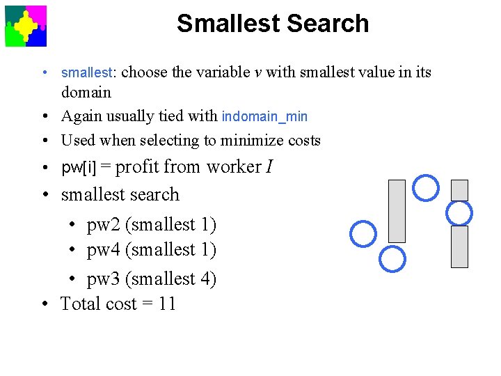
Smallest Search • smallest: choose the variable v with smallest value in its domain • Again usually tied with indomain_min • Used when selecting to minimize costs • pw[i] = profit from worker I • smallest search • pw 2 (smallest 1) • pw 4 (smallest 1) • pw 3 (smallest 4) • Total cost = 11

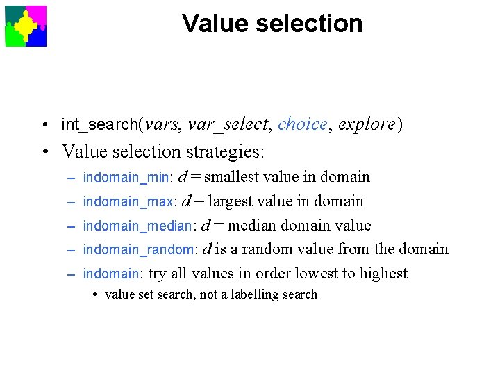
Value selection • int_search(vars, var_select, choice, explore) • Value selection strategies: – indomain_min: d = smallest value in domain – indomain_max: d = largest value in domain – indomain_median: d = median domain value – indomain_random: d is a random value from the domain – indomain: try all values in order lowest to highest • value set search, not a labelling search

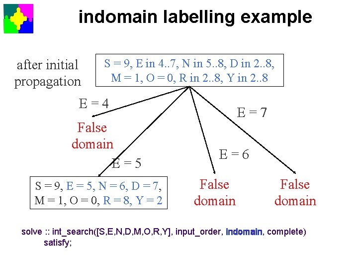
indomain labelling example after initial propagation S = 9, E in 4. . 7, N in 5. . 8, D in 2. . 8, M = 1, O = 0, R in 2. . 8, Y in 2. . 8 E=4 False domain E=5 S = 9, E = 5, N = 6, D = 7, M = 1, O = 0, R = 8, Y = 2 E=7 E=6 False domain solve : : int_search([S, E, N, D, M, O, R, Y], input_order, indomain, complete) satisfy;

Value selection question • What is the difference between – indomain, and – indomain_min ?

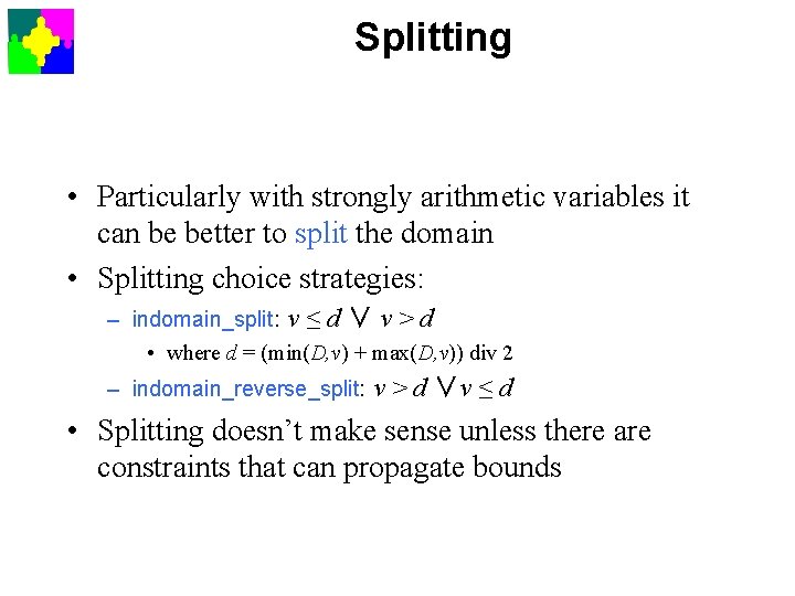
Splitting • Particularly with strongly arithmetic variables it can be better to split the domain • Splitting choice strategies: – indomain_split: v ≤ d ∨ v > d • where d = (min(D, v) + max(D, v)) div 2 – indomain_reverse_split: v > d ∨v ≤ d • Splitting doesn’t make sense unless there are constraints that can propagate bounds

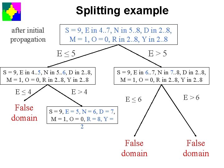
Splitting example after initial propagation S = 9, E in 4. . 7, N in 5. . 8, D in 2. . 8, M = 1, O = 0, R in 2. . 8, Y in 2. . 8 E≤ 5 S = 9, E in 4. . 5, N in 5. . 6, D in 2. . 8, M = 1, O = 0, R in 2. . 8, Y in 2. . 8 E≤ 4 False domain E>4 E>5 S = 9, E in 6. . 7, N in 7. . 8, D in 2. . 8, M = 1, O = 0, R in 2. . 8, Y in 2. . 8 E≤ 6 E>6 S = 9, E = 5, N = 6, D = 7, M = 1, O = 0, R = 8, Y = 2 False domain

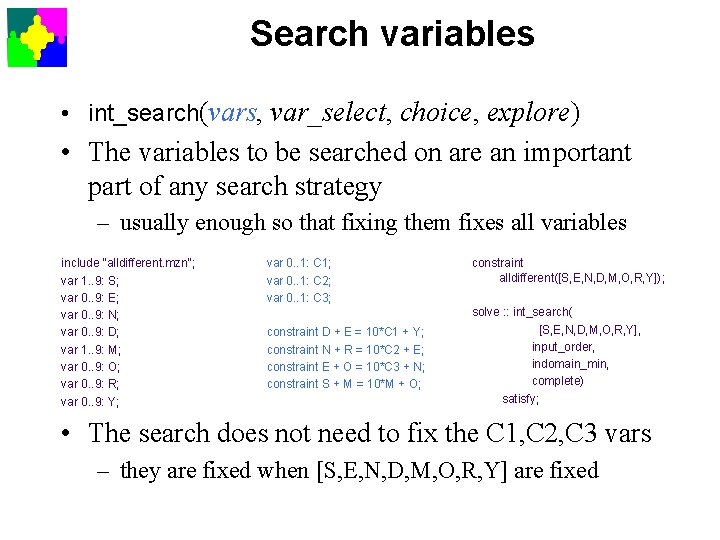
Search variables • int_search(vars, var_select, choice, explore) • The variables to be searched on are an important part of any search strategy – usually enough so that fixing them fixes all variables include "alldifferent. mzn"; var 1. . 9: S; var 0. . 9: E; var 0. . 9: N; var 0. . 9: D; var 1. . 9: M; var 0. . 9: O; var 0. . 9: R; var 0. . 9: Y; var 0. . 1: C 1; var 0. . 1: C 2; var 0. . 1: C 3; constraint D + E = 10*C 1 + Y; constraint N + R = 10*C 2 + E; constraint E + O = 10*C 3 + N; constraint S + M = 10*M + O; constraint alldifferent([S, E, N, D, M, O, R, Y]); solve : : int_search( [S, E, N, D, M, O, R, Y], input_order, indomain_min, complete) satisfy; • The search does not need to fix the C 1, C 2, C 3 vars – they are fixed when [S, E, N, D, M, O, R, Y] are fixed

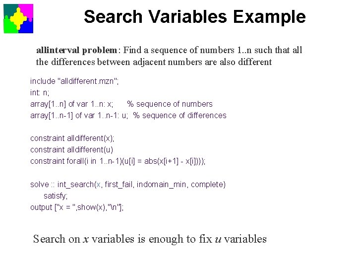
Search Variables Example allinterval problem: Find a sequence of numbers 1. . n such that all the differences between adjacent numbers are also different include "alldifferent. mzn"; int: n; array[1. . n] of var 1. . n: x; % sequence of numbers array[1. . n-1] of var 1. . n-1: u; % sequence of differences constraint alldifferent(x); constraint alldifferent(u) constraint forall(i in 1. . n-1)(u[i] = abs(x[i+1] - x[i]))); solve : : int_search(x, first_fail, indomain_min, complete) satisfy; output ["x = ", show(x), "n"]; Search on x variables is enough to fix u variables

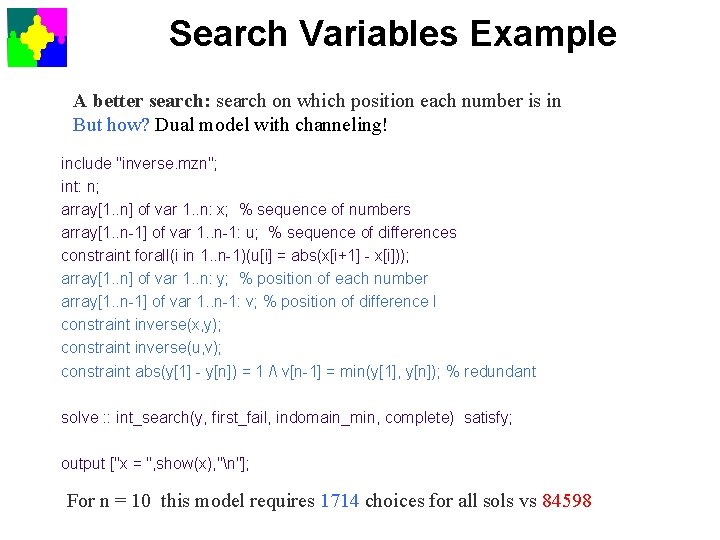
Search Variables Example A better search: search on which position each number is in But how? Dual model with channeling! include "inverse. mzn"; int: n; array[1. . n] of var 1. . n: x; % sequence of numbers array[1. . n-1] of var 1. . n-1: u; % sequence of differences constraint forall(i in 1. . n-1)(u[i] = abs(x[i+1] - x[i])); array[1. . n] of var 1. . n: y; % position of each number array[1. . n-1] of var 1. . n-1: v; % position of difference I constraint inverse(x, y); constraint inverse(u, v); constraint abs(y[1] - y[n]) = 1 / v[n-1] = min(y[1], y[n]); % redundant solve : : int_search(y, first_fail, indomain_min, complete) satisfy; output ["x = ", show(x), "n"]; For n = 10 this model requires 1714 choices for all sols vs 84598

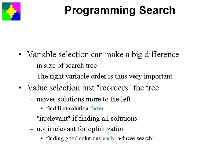
Programming Search • Variable selection can make a big difference – in size of search tree – The right variable order is thus very important • Value selection just "reorders" the tree – moves solutions more to the left • find first solution faster – "irrelevant" if finding all solutions – not irrelevant for optimization • finding good solutions early reduces search!

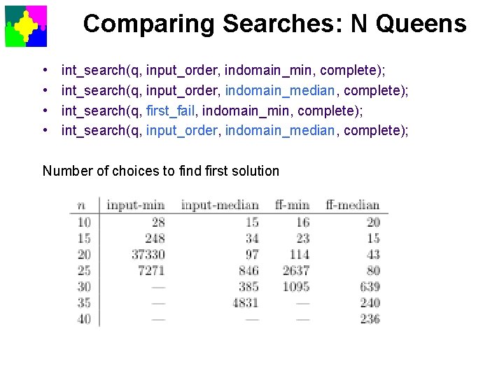
Comparing Searches: N Queens • • int_search(q, input_order, indomain_min, complete); int_search(q, input_order, indomain_median, complete); int_search(q, first_fail, indomain_min, complete); int_search(q, input_order, indomain_median, complete); Number of choices to find first solution

Complex Searches • Actually very many different complex search strategies have been used/defined for FD solvers • Mini. Zinc currently only supports one complex search constructor: sequential search – seq_search( [ search_ann, …, search_ann ]) • Complete the first search before starting the next one.

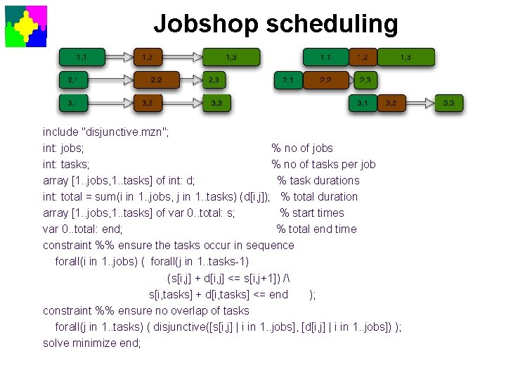
Jobshop scheduling include "disjunctive. mzn"; int: jobs; % no of jobs int: tasks; % no of tasks per job array [1. . jobs, 1. . tasks] of int: d; % task durations int: total = sum(i in 1. . jobs, j in 1. . tasks) (d[i, j]); % total duration array [1. . jobs, 1. . tasks] of var 0. . total: s; % start times var 0. . total: end; % total end time constraint %% ensure the tasks occur in sequence forall(i in 1. . jobs) ( forall(j in 1. . tasks-1) (s[i, j] + d[i, j] <= s[i, j+1]) / s[i, tasks] + d[i, tasks] <= end ); constraint %% ensure no overlap of tasks forall(j in 1. . tasks) ( disjunctive([s[i, j] | i in 1. . jobs], [d[i, j] | i in 1. . jobs]) ); solve minimize end;

Jobshop search strategies • seq_search([ int_search([s[i. j]| i in 1. . jobs, j in 1. . tasks], smallest, indomain_min, complete), int_search([end], input_order, indomain_min, complete) ]) Place earliest tasks first, when finished set end to minimum time! • seq_search([ int_search([end], input_order, indomain_min, complete), int_search([s[i. j]| i in 1. . jobs, j in 1. . tasks], smallest, indomain_min, complete) ]) Optimistic search: Search for a solution with least end time, if that fails search for one higher. Search for solutions using earliest start time.

Annotations • Annotations are how to communicate information to the solver from a Mini. Zinc model – first class object: type ann, annotation variables – can be defined in data files – you can create your own new annotations • annotation <ann-name> ( <arg-def>. . <arg-def> ) ann: search; ann: subsearch = int_search([s[i. j]| i in 1. . jobs, j in 1. . tasks], smallest, indomain_min, complete); solve : : search minimize end; (data file 1) search = subsearch; (data file 2) search = seq_search([subsearch, int_search([end], input_order, indomain_min, complete)]);

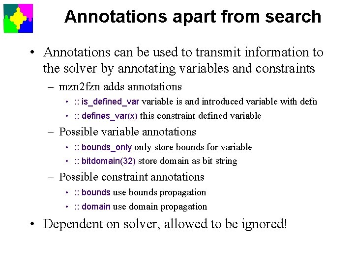
Annotations apart from search • Annotations can be used to transmit information to the solver by annotating variables and constraints – mzn 2 fzn adds annotations • : : is_defined_var variable is and introduced variable with defn • : : defines_var(x) this constraint defined variable – Possible variable annotations • : : bounds_only store bounds for variable • : : bitdomain(32) store domain as bit string – Possible constraint annotations • : : bounds use bounds propagation • : : domain use domain propagation • Dependent on solver, allowed to be ignored!

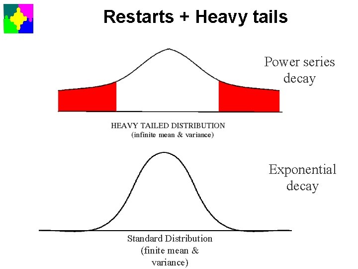
Restarts + Heavy tails Power series decay Exponential decay Standard Distribution (finite mean & variance)

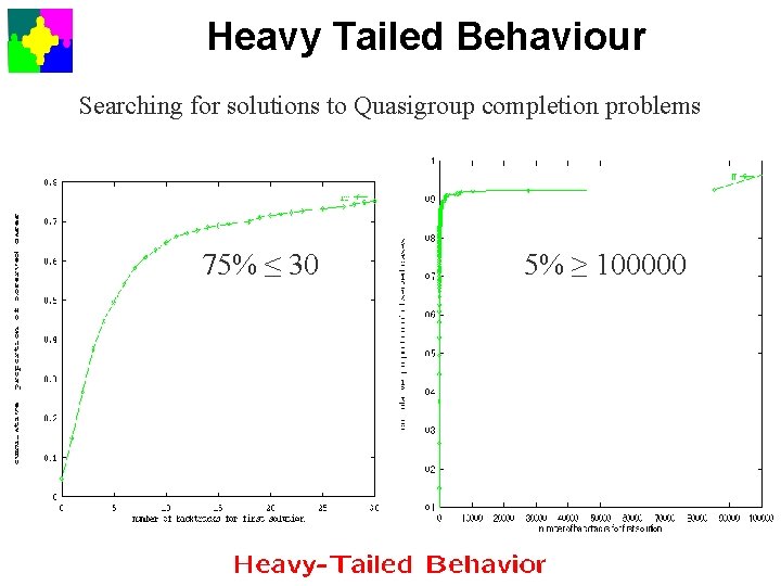
Heavy Tailed Behaviour Searching for solutions to Quasigroup completion problems 75% ≤ 30 5% ≥ 100000

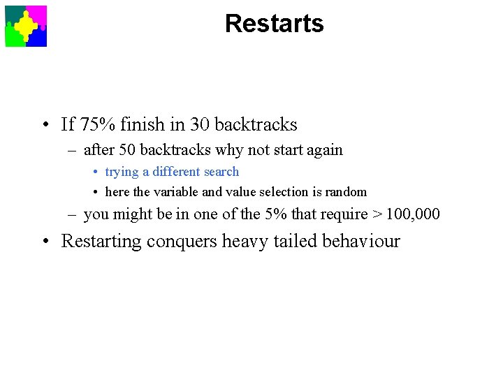
Restarts • If 75% finish in 30 backtracks – after 50 backtracks why not start again • trying a different search • here the variable and value selection is random – you might be in one of the 5% that require > 100, 000 • Restarting conquers heavy tailed behaviour

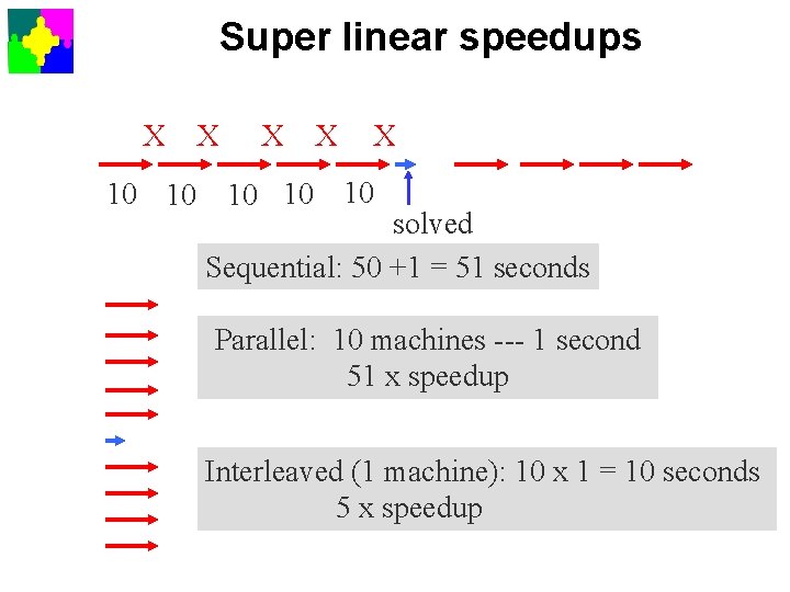
Super linear speedups X 10 10 X X 10 10 10 solved Sequential: 50 +1 = 51 seconds Parallel: 10 machines --- 1 second 51 x speedup Interleaved (1 machine): 10 x 1 = 10 seconds 5 x speedup

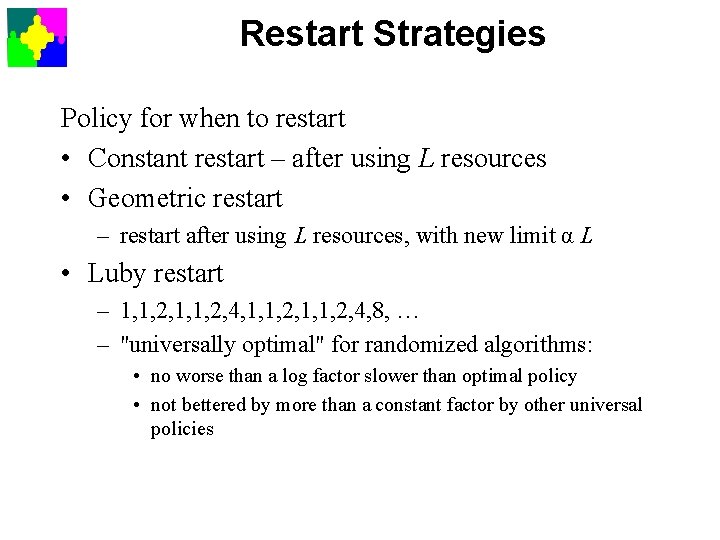
Restart Strategies Policy for when to restart • Constant restart – after using L resources • Geometric restart – restart after using L resources, with new limit α L • Luby restart – 1, 1, 2, 4, 8, … – "universally optimal" for randomized algorithms: • no worse than a log factor slower than optimal policy • not bettered by more than a constant factor by other universal policies

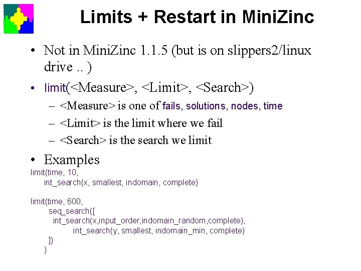
Limits + Restart in Mini. Zinc • Not in Mini. Zinc 1. 1. 5 (but is on slippers 2/linux drive. . ) • limit(<Measure>, <Limit>, <Search>) – <Measure> is one of fails, solutions, nodes, time – <Limit> is the limit where we fail – <Search> is the search we limit • Examples limit(time, 10, int_search(x, smallest, indomain, complete) limit(time, 600, seq_search([ int_search(x, input_order, indomain_random, complete), int_search(y, smallest, indomain_min, complete) ]) )

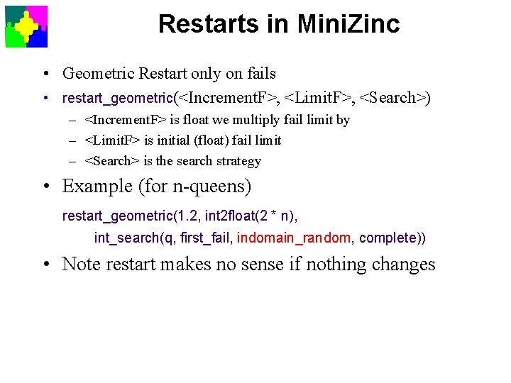
Restarts in Mini. Zinc • Geometric Restart only on fails • restart_geometric(<Increment. F>, <Limit. F>, <Search>) – <Increment. F> is float we multiply fail limit by – <Limit. F> is initial (float) fail limit – <Search> is the search strategy • Example (for n-queens) restart_geometric(1. 2, int 2 float(2 * n), int_search(q, first_fail, indomain_random, complete)) • Note restart makes no sense if nothing changes

Autonomous Search • A highly active research area in constraint programming (all rely on restarting for max effect) • Automatic search strategies examples – dom_w_deg: choose a variable with minimum • domain size / sum of failures caused by constraints it is in – impact: record for each v = d constraint • the average change in product of domain sizes when this choice is made = impact of decision • choose the variable v with maximum impact • choose the value d for v with minimum impact – activity: record for v = d, v ≤ d, v ≥ d, v ≠ d • when it is involved in a failure (requires tracking implications) • decay activities, to focus on more recent failures • choose the constraint with highest activity

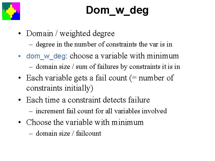
Dom_w_deg • Domain / weighted degree – degree in the number of constraints the var is in • dom_w_deg: choose a variable with minimum – domain size / sum of failures by constraints it is in • Each variable gets a fail count (= number of constraints initially) • Each time a constraint detects failure – increment fail count for all variables involved • Choose the variable with minimum – domain size / failcount

Dom_w_deg • Why does it work include "all_different. mzn”; array[1. . 15] of var 0. . 1: b; array[1. . 4] of var 1. . 10: x; constraint sum(b) >= 1 / exists([b[i] == 1 | i in 1. . 15]); constraint all_different(x) / sum(i in 1. . 4)(x[i]) = 9; solve : : int_search(b++x, first_fail, indomain_min, complete) satisfy; – 491504 choices to fail • Change to dom_w_deg – 182 choices to fail • first branch choose bs then xs • since all failure is on xs we never rechoose a b on backtracking

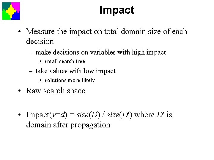
Impact • Measure the impact on total domain size of each decision – make decisions on variables with high impact • small search tree – take values with low impact • solutions more likely • Raw search space • Impact(v=d) = size(D) / size(D') where D' is domain after propagation

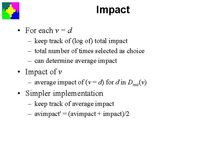
Impact • For each v = d – keep track of (log of) total impact – total number of times selected as choice – can determine average impact • Impact of v – average impact of (v = d) for d in Dinit(v) • Simpler implementation – keep track of average impact – avimpact' = (avimpact + impact)/2

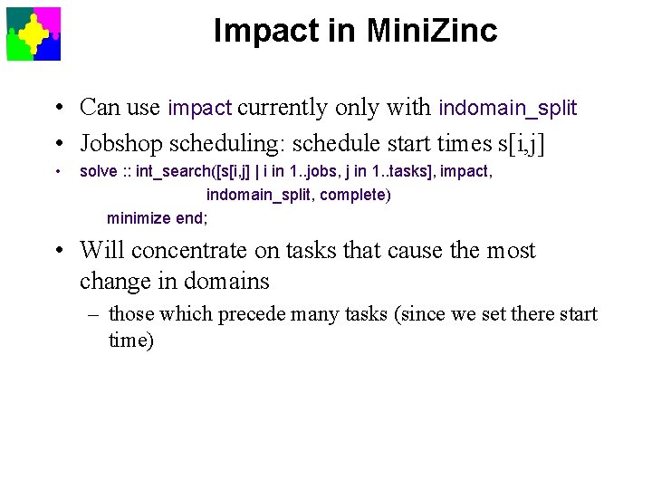
Impact in Mini. Zinc • Can use impact currently only with indomain_split • Jobshop scheduling: schedule start times s[i, j] • solve : : int_search([s[i, j] | i in 1. . jobs, j in 1. . tasks], impact, indomain_split, complete) minimize end; • Will concentrate on tasks that cause the most change in domains – those which precede many tasks (since we set there start time)

Activity-based Search • We will examine after we have studied – Boolean Satisfiability Search where it was devised.

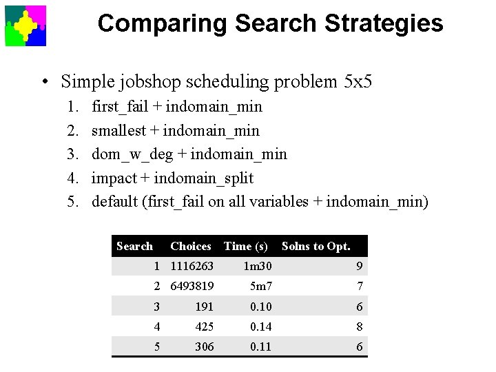
Comparing Search Strategies • Simple jobshop scheduling problem 5 x 5 1. 2. 3. 4. 5. first_fail + indomain_min smallest + indomain_min dom_w_deg + indomain_min impact + indomain_split default (first_fail on all variables + indomain_min) Search Choices Time (s) Solns to Opt. 1 1116263 1 m 30 9 2 6493819 5 m 7 7 3 191 0. 10 6 4 425 0. 14 8 5 306 0. 11 6

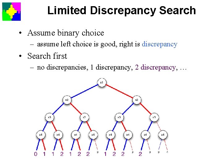
Limited Discrepancy Search • Programmed search difficulties – most important decisions at top of tree – where least information is available • Restarting fixes this to some degree – restart with better information • Restarting usually changes the order of variables selected • What about changing the order of values selected?

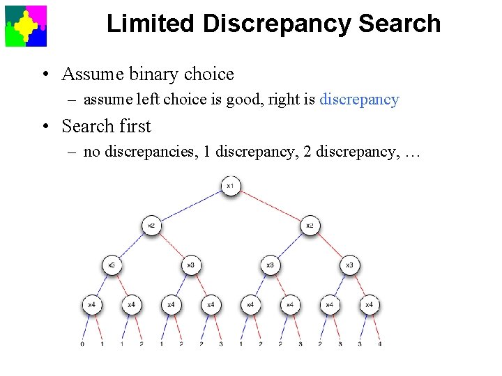
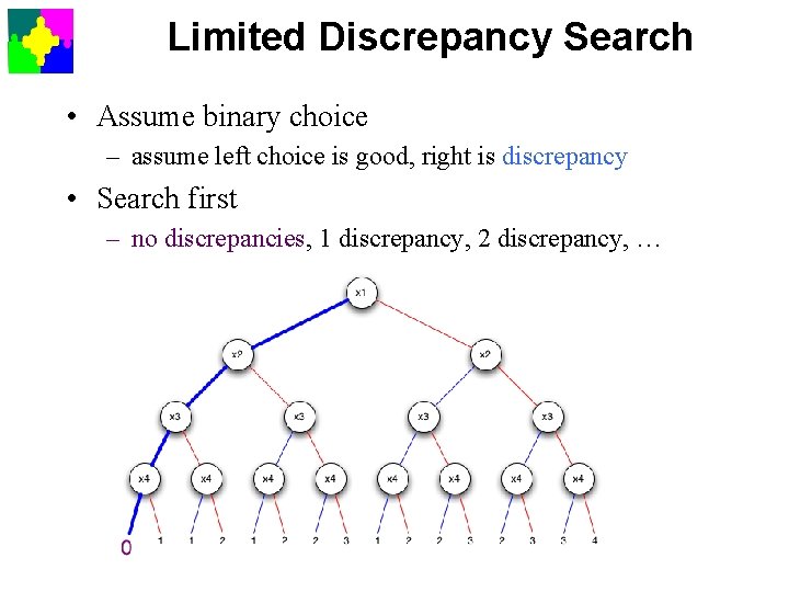
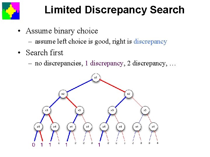
Limited Discrepancy Search • Assume binary choice – assume left choice is good, right is discrepancy • Search first – no discrepancies, 1 discrepancy, 2 discrepancy, …

Limited Discrepancy Search • Assume binary choice – assume left choice is good, right is discrepancy • Search first – no discrepancies, 1 discrepancy, 2 discrepancy, …

Limited Discrepancy Search • Assume binary choice – assume left choice is good, right is discrepancy • Search first – no discrepancies, 1 discrepancy, 2 discrepancy, …

Limited Discrepancy Search • Assume binary choice – assume left choice is good, right is discrepancy • Search first – no discrepancies, 1 discrepancy, 2 discrepancy, …

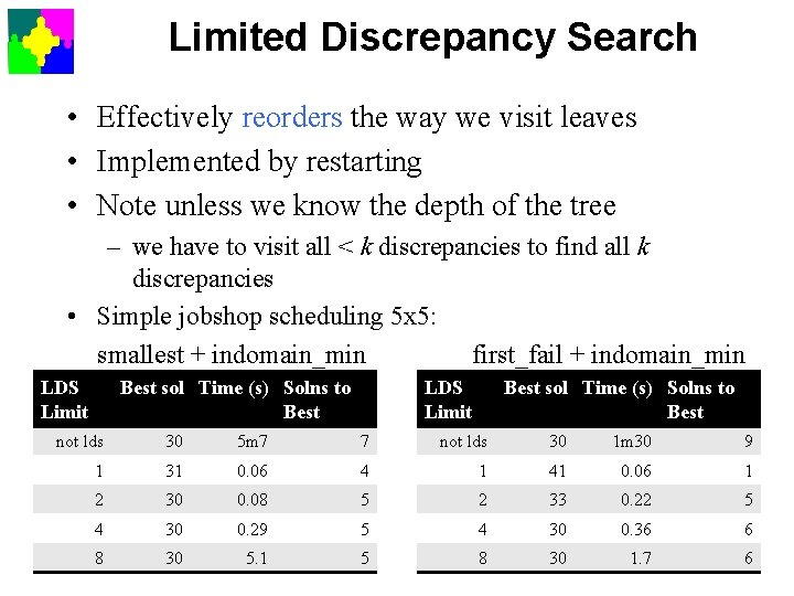
Limited Discrepancy Search • Effectively reorders the way we visit leaves • Implemented by restarting • Note unless we know the depth of the tree – we have to visit all < k discrepancies to find all k discrepancies • Simple jobshop scheduling 5 x 5: smallest + indomain_min first_fail + indomain_min LDS Limit Best sol Time (s) Solns to Best not lds 30 5 m 7 7 not lds 30 1 m 30 9 1 31 0. 06 4 1 41 0. 06 1 2 30 0. 08 5 2 33 0. 22 5 4 30 0. 29 5 4 30 0. 36 6 8 30 5. 1 5 8 30 1. 7 6

Summary • Constraint programming techniques are based on backtracking search • Reduce the search using consistency methods – incomplete but faster – node, arc, bound, generalized • Optimization can be based on a branch & bound with a backtracking search • Very general approach, not restricted to linear constraints. • Programmer can add new global constraints and program their propagation behaviour.

Exercise 1: Send-most-money • The send-most-money problem is to find different digits that make the cryptarithmetic problem: SEND + MOST = MONEY hold while maximizing MONEY (ie. 10000*M+ 1000*O+100*N_10*E+Y) • Write a Mini. Zinc model and try out different search strategies to solve it. Which requires the least choices?