Programming Languages CSCI 44306430 Part 1 Functional Programming

Programming Languages (CSCI 4430/6430) Part 1: Functional Programming: Summary Carlos Varela Rennselaer Polytechnic Institute September 29, 2015 C. Varela 1

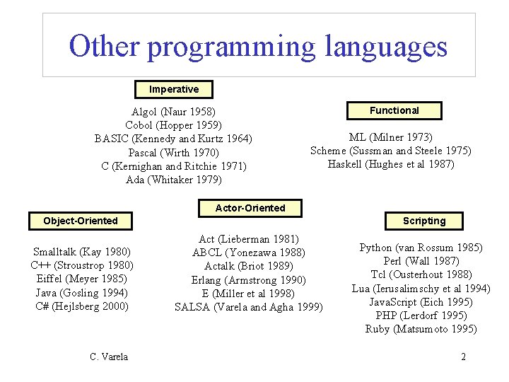
Other programming languages Imperative Algol (Naur 1958) Cobol (Hopper 1959) BASIC (Kennedy and Kurtz 1964) Pascal (Wirth 1970) C (Kernighan and Ritchie 1971) Ada (Whitaker 1979) Functional ML (Milner 1973) Scheme (Sussman and Steele 1975) Haskell (Hughes et al 1987) Actor-Oriented Object-Oriented Smalltalk (Kay 1980) C++ (Stroustrop 1980) Eiffel (Meyer 1985) Java (Gosling 1994) C# (Hejlsberg 2000) C. Varela Scripting Act (Lieberman 1981) ABCL (Yonezawa 1988) Actalk (Briot 1989) Erlang (Armstrong 1990) E (Miller et al 1998) SALSA (Varela and Agha 1999) Python (van Rossum 1985) Perl (Wall 1987) Tcl (Ousterhout 1988) Lua (Ierusalimschy et al 1994) Java. Script (Eich 1995) PHP (Lerdorf 1995) Ruby (Matsumoto 1995) 2

Language syntax • Defines what are the legal programs, i. e. programs that can be executed by a machine (interpreter) • Syntax is defined by grammar rules • A grammar defines how to make ‘sentences’ out of ‘words’ • For programming languages: sentences are called statements (commands, expressions) • For programming languages: words are called tokens • Grammar rules are used to describe both tokens and statements C. Varela; Adapted w/permission from S. Haridi and P. Van Roy 3

Language Semantics • Semantics defines what a program does when it executes • Semantics should be simple and yet allows reasoning about programs (correctness, execution time, and memory use) C. Varela; Adapted w/permission from S. Haridi and P. Van Roy 4

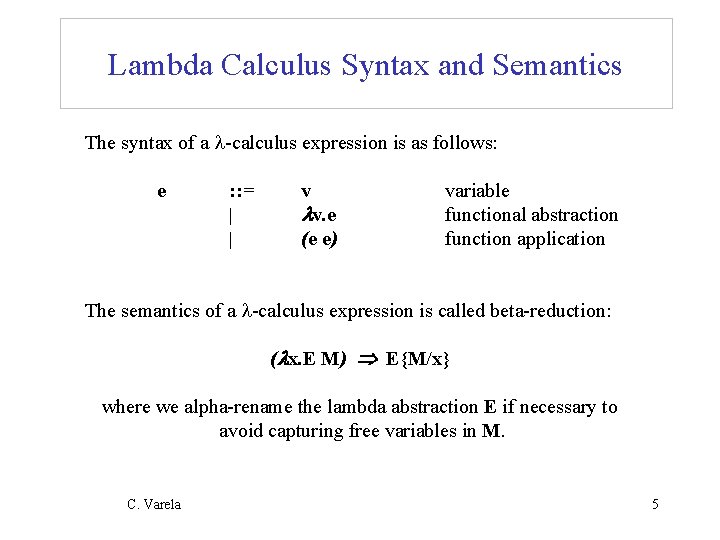
Lambda Calculus Syntax and Semantics The syntax of a -calculus expression is as follows: e : : = | | v v. e (e e) variable functional abstraction function application The semantics of a -calculus expression is called beta-reduction: ( x. E M) E{M/x} where we alpha-rename the lambda abstraction E if necessary to avoid capturing free variables in M. C. Varela 5

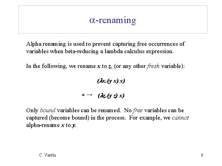
-renaming Alpha renaming is used to prevent capturing free occurrences of variables when beta-reducing a lambda calculus expression. In the following, we rename x to z, (or any other fresh variable): ( x. (y x) x) α → ( z. (y z) x) Only bound variables can be renamed. No free variables can be captured (become bound) in the process. For example, we cannot alpha-rename x to y. C. Varela 6

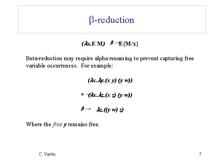
b-reduction ( x. E M) b →E{M/x} Beta-reduction may require alpha renaming to prevent capturing free variable occurrences. For example: ( x. y. (x y) (y w)) α → ( x. z. (x z) (y w)) b → z. ((y w) z) Where the free y remains free. C. Varela 7

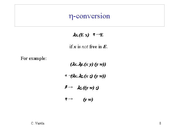
h-conversion x. (E x) h →E if x is not free in E. For example: ( x. y. (x y) (y w)) α → ( x. z. (x z) (y w)) b → z. ((y w) z) h→ C. Varela (y w) 8

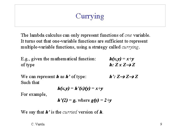
Currying The lambda calculus can only represent functions of one variable. It turns out that one-variable functions are sufficient to represent multiple-variable functions, using a strategy called currying. E. g. , given the mathematical function: of type h(x, y) = x+y h: Z x Z Z We can represent h as h’ of type: h’: Z Z Z Such that h(x, y) = h’(x)(y) = x+y For example, h’(2) = g, where g(y) = 2+y We say that h’ is the curried version of h. C. Varela 9

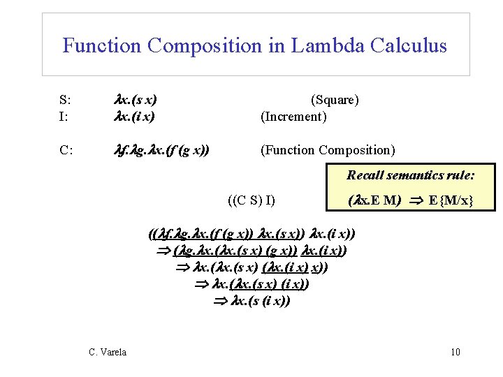
Function Composition in Lambda Calculus S: I: x. (s x) x. (i x) (Square) (Increment) C: f. g. x. (f (g x)) (Function Composition) Recall semantics rule: ((C S) I) ( x. E M) E{M/x} (( f. g. x. (f (g x)) x. (s x)) x. (i x)) ( g. x. (s x) (g x)) x. (i x)) x. (s x) ( x. (i x) x)) x. (s x) (i x)) x. (s (i x)) C. Varela 10

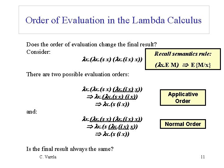
Order of Evaluation in the Lambda Calculus Does the order of evaluation change the final result? Consider: Recall semantics rule: x. (s x) ( x. (i x) x)) ( x. E M) E{M/x} There are two possible evaluation orders: and: x. (s x) ( x. (i x) x)) x. (s x) (i x)) x. (s (i x)) Applicative Order x. (s x) ( x. (i x) x)) x. (s (i x)) Normal Order Is the final result always the same? C. Varela 11

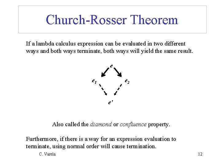
Church-Rosser Theorem If a lambda calculus expression can be evaluated in two different ways and both ways terminate, both ways will yield the same result. e e 1 e 2 e’ Also called the diamond or confluence property. Furthermore, if there is a way for an expression evaluation to terminate, using normal order will cause termination. C. Varela 12

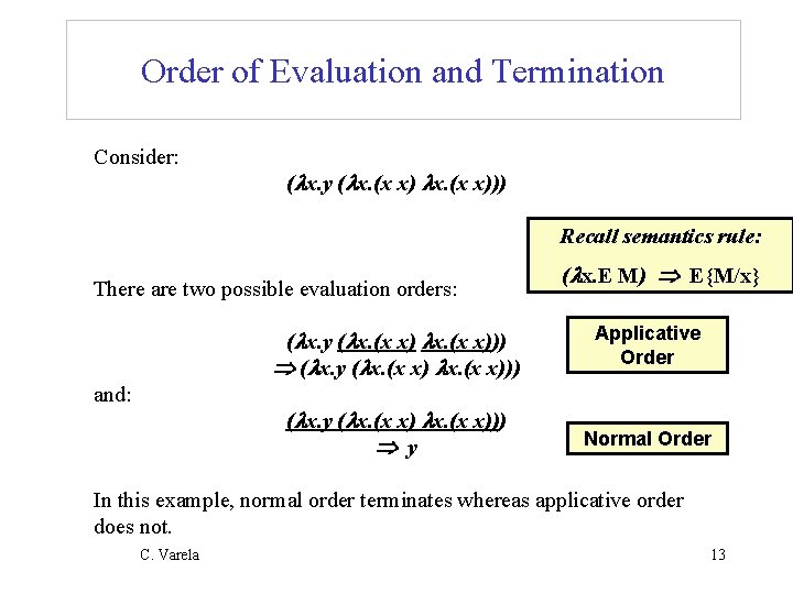
Order of Evaluation and Termination Consider: ( x. y ( x. (x x))) Recall semantics rule: There are two possible evaluation orders: and: ( x. E M) E{M/x} ( x. y ( x. (x x))) Applicative Order ( x. y ( x. (x x))) y Normal Order In this example, normal order terminates whereas applicative order does not. C. Varela 13

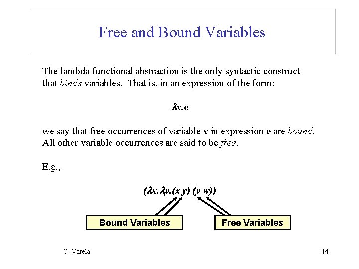
Free and Bound Variables The lambda functional abstraction is the only syntactic construct that binds variables. That is, in an expression of the form: v. e we say that free occurrences of variable v in expression e are bound. All other variable occurrences are said to be free. E. g. , ( x. y. (x y) (y w)) Bound Variables C. Varela Free Variables 14

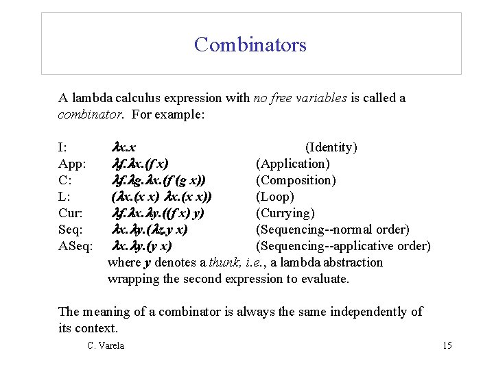
Combinators A lambda calculus expression with no free variables is called a combinator. For example: I: App: C: L: Cur: Seq: ASeq: x. x (Identity) f. x. (f x) (Application) f. g. x. (f (g x)) (Composition) ( x. (x x)) (Loop) f. x. y. ((f x) y) (Currying) x. y. ( z. y x) (Sequencing--normal order) x. y. (y x) (Sequencing--applicative order) where y denotes a thunk, i. e. , a lambda abstraction wrapping the second expression to evaluate. The meaning of a combinator is always the same independently of its context. C. Varela 15

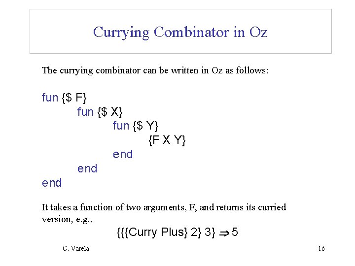
Currying Combinator in Oz The currying combinator can be written in Oz as follows: fun {$ F} fun {$ X} fun {$ Y} {F X Y} end end It takes a function of two arguments, F, and returns its curried version, e. g. , {{{Curry Plus} 2} 3} 5 C. Varela 16

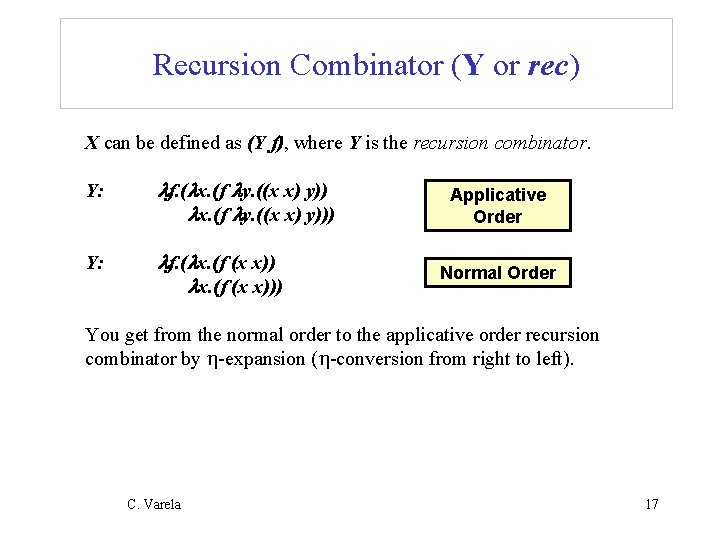
Recursion Combinator (Y or rec) X can be defined as (Y f), where Y is the recursion combinator. Y: f. ( x. (f y. ((x x) y))) Y: f. ( x. (f (x x))) Applicative Order Normal Order You get from the normal order to the applicative order recursion combinator by h-expansion (h-conversion from right to left). C. Varela 17

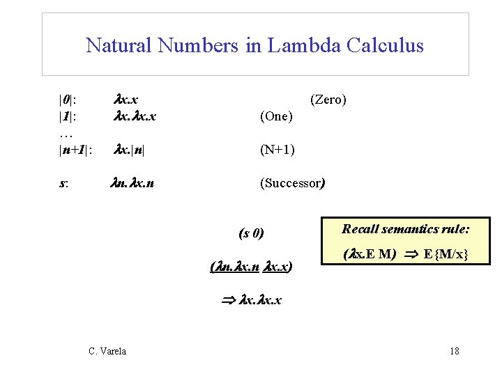
Natural Numbers in Lambda Calculus |0|: |1|: … |n+1|: x. x. x (One) x. |n| (N+1) s: n. x. n (Successor) (Zero) (s 0) ( n. x. n x. x) Recall semantics rule: ( x. E M) E{M/x} x. x. x C. Varela 18

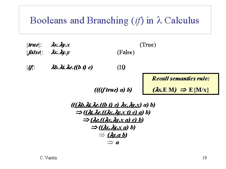
Booleans and Branching (if) in Calculus |true|: x. y. x |false|: x. y. y |if|: (True) (False) b. t. e. ((b t) e) (If) Recall semantics rule: (((if true) a) b) ( x. E M) E{M/x} ((( b. t. e. ((b t) e) x. y. x) a) b) (( t. e. (( x. y. x t) e) a) b) ( e. (( x. y. x a) e) b) (( x. y. x a) b) Þ ( y. a b) Þa C. Varela 19

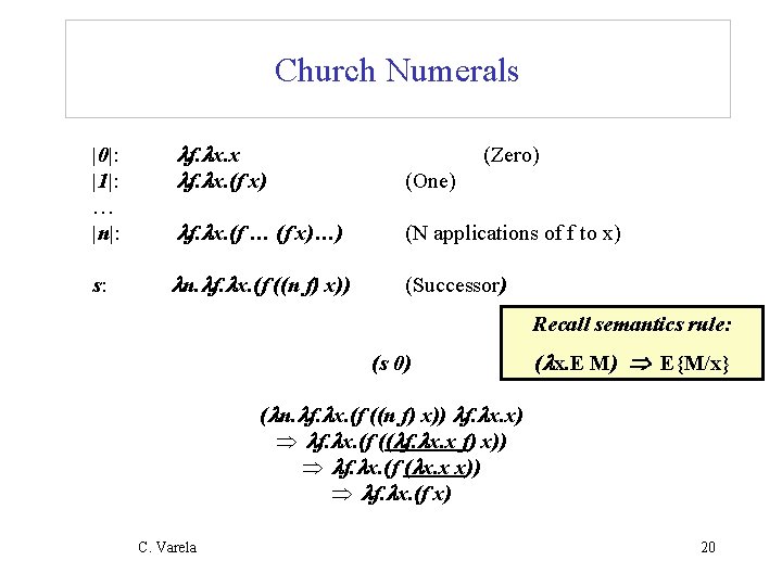
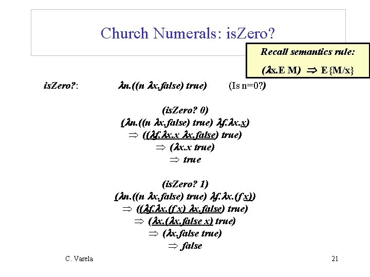
Church Numerals |0|: |1|: … |n|: f. x. x f. x. (f x) (One) f. x. (f … (f x)…) (N applications of f to x) s: n. f. x. (f ((n f) x)) (Successor) (Zero) Recall semantics rule: (s 0) ( x. E M) E{M/x} ( n. f. x. (f ((n f) x)) f. x. x) Þ f. x. (f (( f. x. x f) x)) Þ f. x. (f ( x. x x)) Þ f. x. (f x) C. Varela 20

Church Numerals: is. Zero? Recall semantics rule: is. Zero? : n. ((n x. false) true) ( x. E M) E{M/x} (Is n=0? ) (is. Zero? 0) ( n. ((n x. false) true) f. x. x) Þ (( f. x. x x. false) true) Þ ( x. x true) Þ true (is. Zero? 1) ( n. ((n x. false) true) f. x. (f x)) Þ (( f. x. (f x) x. false) true) Þ ( x. false x) true) Þ ( x. false true) Þ false C. Varela 21

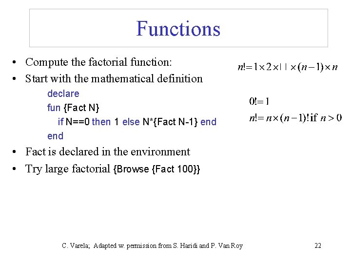
Functions • Compute the factorial function: • Start with the mathematical definition declare fun {Fact N} if N==0 then 1 else N*{Fact N-1} end • Fact is declared in the environment • Try large factorial {Browse {Fact 100}} C. Varela; Adapted w. permission from S. Haridi and P. Van Roy 22

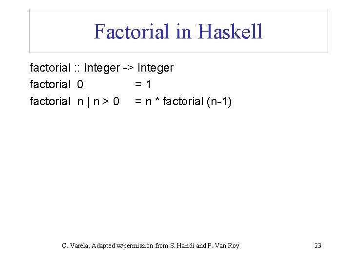
Factorial in Haskell factorial : : Integer -> Integer factorial 0 =1 factorial n | n > 0 = n * factorial (n-1) C. Varela; Adapted w/permission from S. Haridi and P. Van Roy 23

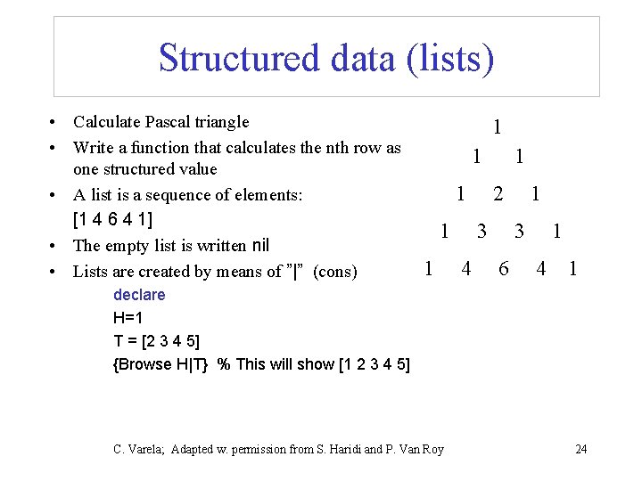
Structured data (lists) • Calculate Pascal triangle • Write a function that calculates the nth row as one structured value • A list is a sequence of elements: [1 4 6 4 1] • The empty list is written nil • Lists are created by means of ”|” (cons) 1 1 1 2 3 4 1 3 6 1 4 1 declare H=1 T = [2 3 4 5] {Browse H|T} % This will show [1 2 3 4 5] C. Varela; Adapted w. permission from S. Haridi and P. Van Roy 24

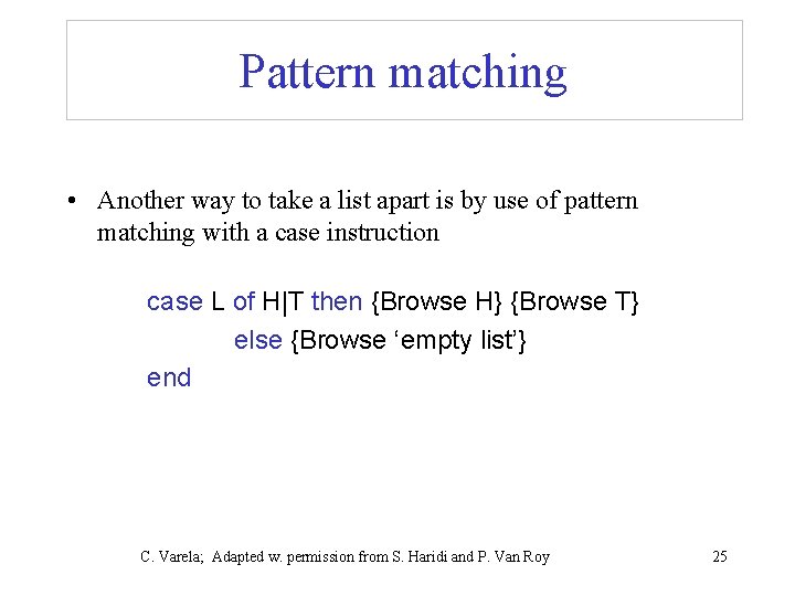
Pattern matching • Another way to take a list apart is by use of pattern matching with a case instruction case L of H|T then {Browse H} {Browse T} else {Browse ‘empty list’} end C. Varela; Adapted w. permission from S. Haridi and P. Van Roy 25

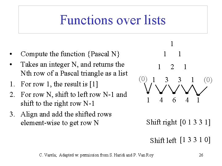
Functions over lists 1 • • Compute the function {Pascal N} Takes an integer N, and returns the Nth row of a Pascal triangle as a list 1. For row 1, the result is [1] 2. For row N, shift to left row N-1 and shift to the right row N-1 3. Align and add the shifted rows element-wise to get row N 1 1 (0) 1 1 1 2 3 4 1 3 6 1 4 (0) 1 Shift right [0 1 3 3 1] Shift left [1 3 3 1 0] C. Varela; Adapted w. permission from S. Haridi and P. Van Roy 26

Functions over lists Pascal N declare fun {Pascal N} if N==1 then [1] else {Add. List {Shift. Left {Pascal N-1}} {Shift. Right {Pascal N 1}}} end Pascal N-1 Shift. Left Shift. Right C. Varela; Adapted w. permission from S. Haridi and P. Van Roy Add. List 27

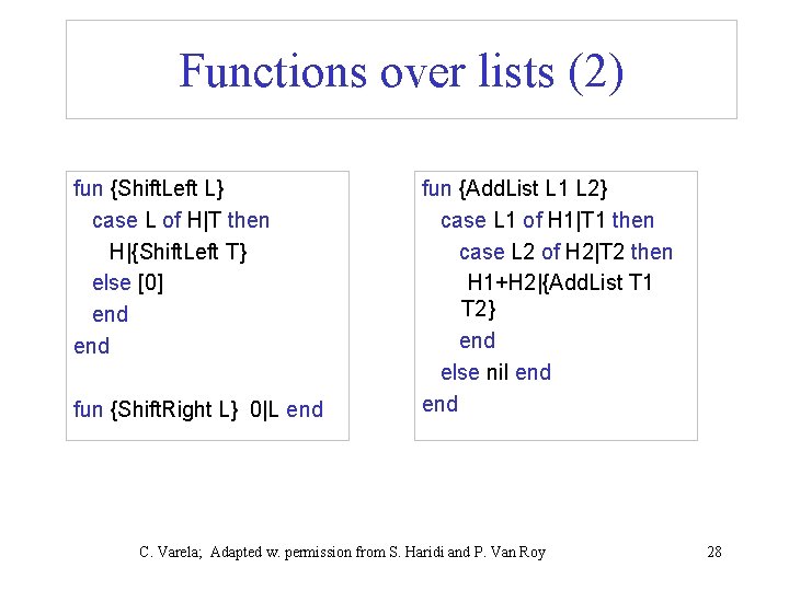
Functions over lists (2) fun {Shift. Left L} case L of H|T then H|{Shift. Left T} else [0] end fun {Shift. Right L} 0|L end fun {Add. List L 1 L 2} case L 1 of H 1|T 1 then case L 2 of H 2|T 2 then H 1+H 2|{Add. List T 1 T 2} end else nil end C. Varela; Adapted w. permission from S. Haridi and P. Van Roy 28

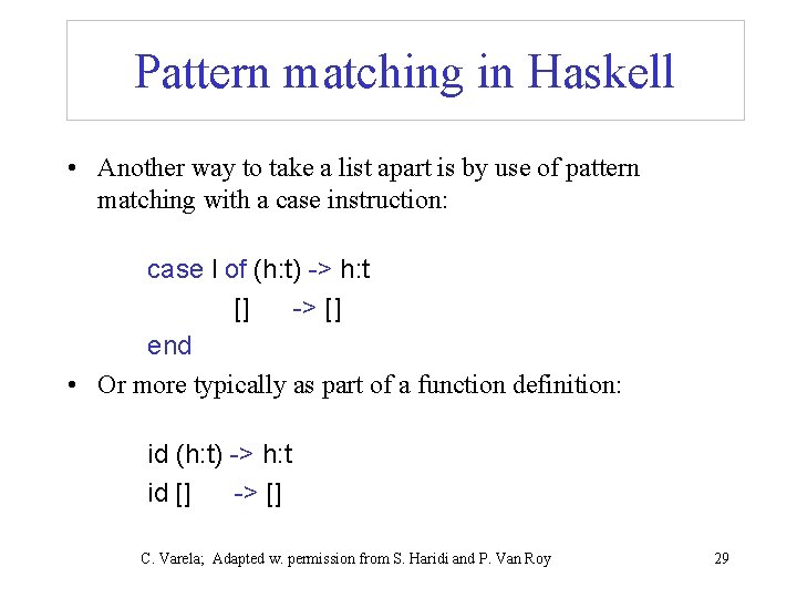
Pattern matching in Haskell • Another way to take a list apart is by use of pattern matching with a case instruction: case l of (h: t) -> h: t [] -> [] end • Or more typically as part of a function definition: id (h: t) -> h: t id [] -> [] C. Varela; Adapted w. permission from S. Haridi and P. Van Roy 29

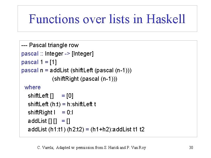
Functions over lists in Haskell --- Pascal triangle row pascal : : Integer -> [Integer] pascal 1 = [1] pascal n = add. List (shift. Left (pascal (n-1))) (shift. Right (pascal (n-1))) where shift. Left [] = [0] shift. Left (h: t) = h: shift. Left t shift. Right l = 0: l add. List [] [] = [] add. List (h 1: t 1) (h 2: t 2) = (h 1+h 2): add. List t 1 t 2 C. Varela; Adapted w. permission from S. Haridi and P. Van Roy 30

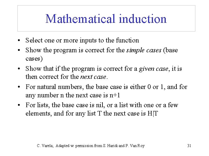
Mathematical induction • Select one or more inputs to the function • Show the program is correct for the simple cases (base cases) • Show that if the program is correct for a given case, it is then correct for the next case. • For natural numbers, the base case is either 0 or 1, and for any number n the next case is n+1 • For lists, the base case is nil, or a list with one or a few elements, and for any list T the next case is H|T C. Varela; Adapted w. permission from S. Haridi and P. Van Roy 31

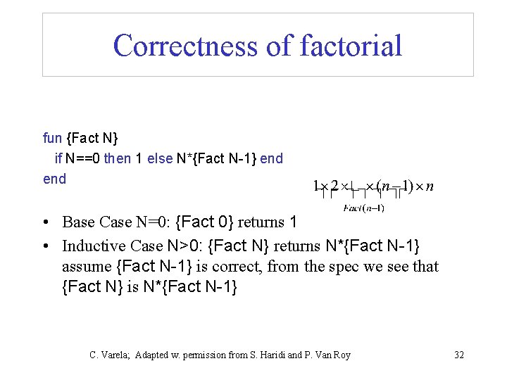
Correctness of factorial fun {Fact N} if N==0 then 1 else N*{Fact N-1} end • Base Case N=0: {Fact 0} returns 1 • Inductive Case N>0: {Fact N} returns N*{Fact N-1} assume {Fact N-1} is correct, from the spec we see that {Fact N} is N*{Fact N-1} C. Varela; Adapted w. permission from S. Haridi and P. Van Roy 32

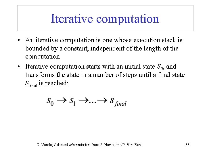
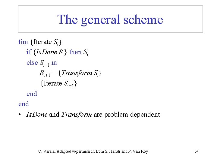
Iterative computation • An iterative computation is one whose execution stack is bounded by a constant, independent of the length of the computation • Iterative computation starts with an initial state S 0, and transforms the state in a number of steps until a final state Sfinal is reached: C. Varela; Adapted w/permission from S. Haridi and P. Van Roy 33

The general scheme fun {Iterate Si} if {Is. Done Si} then Si else Si+1 in Si+1 = {Transform Si} {Iterate Si+1} end • Is. Done and Transform are problem dependent C. Varela; Adapted w/permission from S. Haridi and P. Van Roy 34

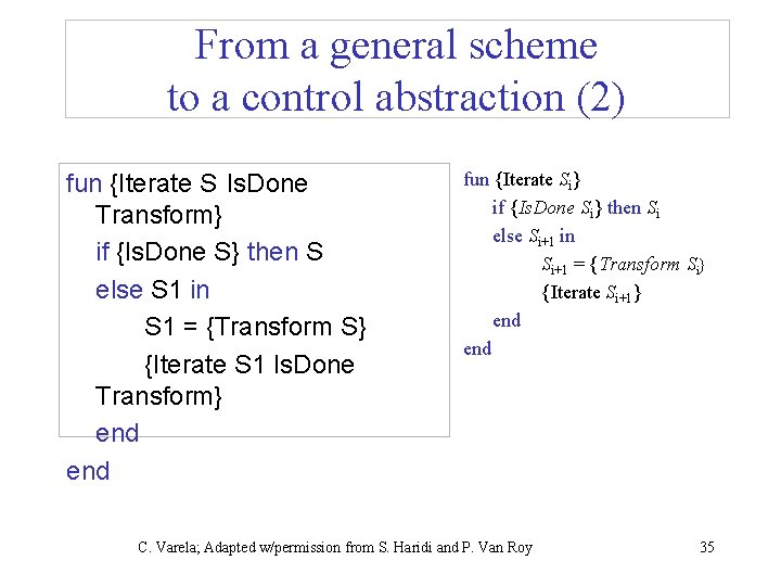
From a general scheme to a control abstraction (2) fun {Iterate S Is. Done Transform} if {Is. Done S} then S else S 1 in S 1 = {Transform S} {Iterate S 1 Is. Done Transform} end fun {Iterate Si} if {Is. Done Si} then Si else Si+1 in Si+1 = {Transform Si} {Iterate Si+1} end C. Varela; Adapted w/permission from S. Haridi and P. Van Roy 35

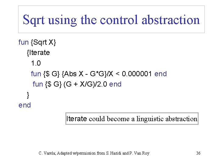
Sqrt using the control abstraction fun {Sqrt X} {Iterate 1. 0 fun {$ G} {Abs X - G*G}/X < 0. 000001 end fun {$ G} (G + X/G)/2. 0 end } end Iterate could become a linguistic abstraction C. Varela; Adapted w/permission from S. Haridi and P. Van Roy 36

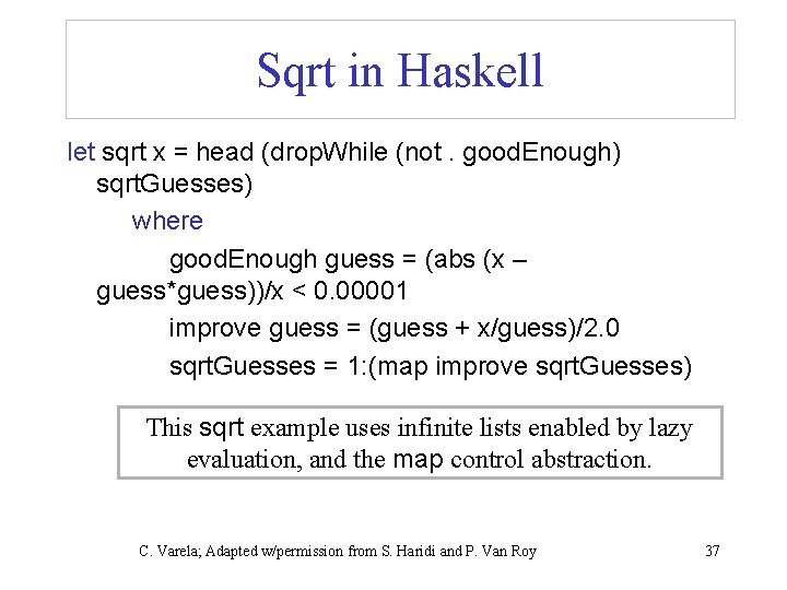
Sqrt in Haskell let sqrt x = head (drop. While (not. good. Enough) sqrt. Guesses) where good. Enough guess = (abs (x – guess*guess))/x < 0. 00001 improve guess = (guess + x/guess)/2. 0 sqrt. Guesses = 1: (map improve sqrt. Guesses) This sqrt example uses infinite lists enabled by lazy evaluation, and the map control abstraction. C. Varela; Adapted w/permission from S. Haridi and P. Van Roy 37

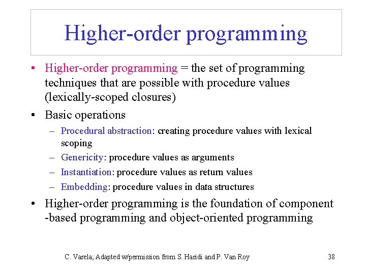
Higher-order programming • Higher-order programming = the set of programming techniques that are possible with procedure values (lexically-scoped closures) • Basic operations – Procedural abstraction: creating procedure values with lexical scoping – Genericity: procedure values as arguments – Instantiation: procedure values as return values – Embedding: procedure values in data structures • Higher-order programming is the foundation of component -based programming and object-oriented programming C. Varela; Adapted w/permission from S. Haridi and P. Van Roy 38

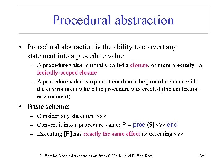
Procedural abstraction • Procedural abstraction is the ability to convert any statement into a procedure value – A procedure value is usually called a closure, or more precisely, a lexically-scoped closure – A procedure value is a pair: it combines the procedure code with the environment where the procedure was created (the contextual environment) • Basic scheme: – Consider any statement <s> – Convert it into a procedure value: P = proc {$} <s> end – Executing {P} has exactly the same effect as executing <s> C. Varela; Adapted w/permission from S. Haridi and P. Van Roy 39

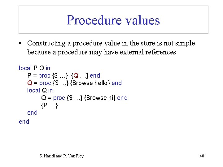
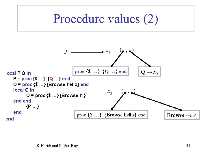
Procedure values • Constructing a procedure value in the store is not simple because a procedure may have external references local P Q in P = proc {$ …} {Q …} end Q = proc {$ …} {Browse hello} end local Q in Q = proc {$ …} {Browse hi} end {P …} end S. Haridi and P. Van Roy 40

Procedure values (2) P x 1 ( , ) proc {$ …} {Q …} end Q x 2 local P Q in P = proc {$ …} {Q …} end Q = proc {$ …} {Browse hello} end local Q in ( , ) x 2 Q = proc {$ …} {Browse hi} end {P …} end proc {$ …} {Browse hello} end S. Haridi and P. Van Roy Browse x 0 41

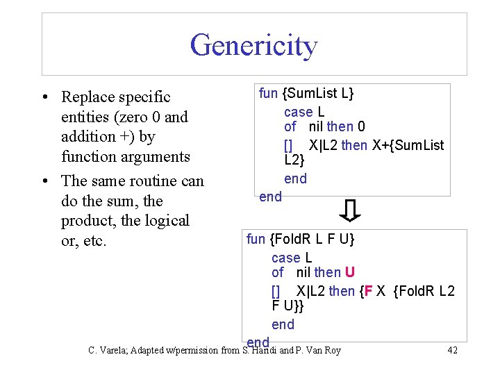
Genericity • Replace specific entities (zero 0 and addition +) by function arguments • The same routine can do the sum, the product, the logical or, etc. fun {Sum. List L} case L of nil then 0 [] X|L 2 then X+{Sum. List L 2} end fun {Fold. R L F U} case L of nil then U [] X|L 2 then {F X {Fold. R L 2 F U}} end C. Varela; Adapted w/permission from S. Haridi and P. Van Roy 42

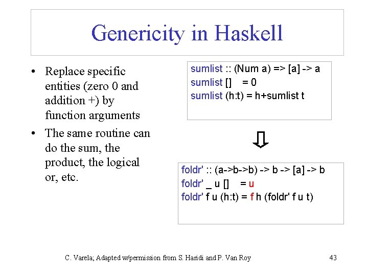
Genericity in Haskell • Replace specific entities (zero 0 and addition +) by function arguments • The same routine can do the sum, the product, the logical or, etc. sumlist : : (Num a) => [a] -> a sumlist [] = 0 sumlist (h: t) = h+sumlist t foldr' : : (a->b->b) -> b -> [a] -> b foldr' _ u [] = u foldr' f u (h: t) = f h (foldr' f u t) C. Varela; Adapted w/permission from S. Haridi and P. Van Roy 43

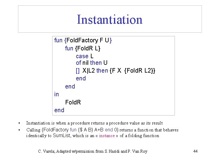
Instantiation fun {Fold. Factory F U} fun {Fold. R L} case L of nil then U [] X|L 2 then {F X {Fold. R L 2}} end in Fold. R end • • Instantiation is when a procedure returns a procedure value as its result Calling {Fold. Factory fun {$ A B} A+B end 0} returns a function that behaves identically to Sum. List, which is an « instance » of a folding function C. Varela; Adapted w/permission from S. Haridi and P. Van Roy 44

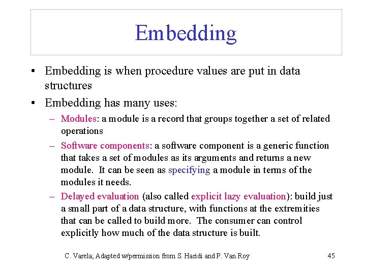
Embedding • Embedding is when procedure values are put in data structures • Embedding has many uses: – Modules: a module is a record that groups together a set of related operations – Software components: a software component is a generic function that takes a set of modules as its arguments and returns a new module. It can be seen as specifying a module in terms of the modules it needs. – Delayed evaluation (also called explicit lazy evaluation): build just a small part of a data structure, with functions at the extremities that can be called to build more. The consumer can control explicitly how much of the data structure is built. C. Varela; Adapted w/permission from S. Haridi and P. Van Roy 45

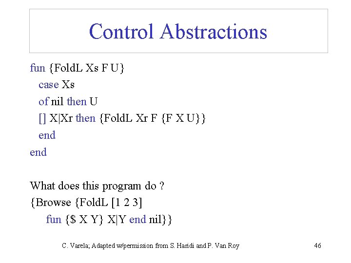
Control Abstractions fun {Fold. L Xs F U} case Xs of nil then U [] X|Xr then {Fold. L Xr F {F X U}} end What does this program do ? {Browse {Fold. L [1 2 3] fun {$ X Y} X|Y end nil}} C. Varela; Adapted w/permission from S. Haridi and P. Van Roy 46

Fold. L in Haskell foldl' : : (b->a->b) -> b -> [a] -> b foldl' _ u [] = u foldl' f u (h: t) = foldl' f (f u h) t Notice the unit u is of type b, and the function f is of type b->a->b. C. Varela; Adapted w/permission from S. Haridi and P. Van Roy 47

List-based techniques fun {Map Xs F} case Xs of nil then nil [] X|Xr then {F X}|{Map Xr F} end fun {Filter Xs P} case Xs of nil then nil [] X|Xr andthen {P X} then X|{Filter Xr P} [] X|Xr then {Filter Xr P} end C. Varela; Adapted w/permission from S. Haridi and P. Van Roy 48

Map in Haskell map' : : (a -> b) -> [a] -> [b] map' _ [] = [] map' f (h: t) = f h: map' f t _ means that the argument is not used (read “don’t care”). map’ is to distinguish it from the Prelude map function. C. Varela; Adapted w/permission from S. Haridi and P. Van Roy 49

Filter in Haskell filter' : : (a-> Bool) -> [a] filter' _ [] = [] filter' p (h: t) = if p h then h: filter' p t else filter' p t C. Varela; Adapted w/permission from S. Haridi and P. Van Roy 50

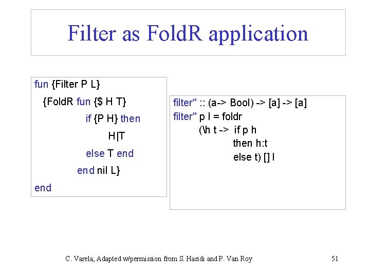
Filter as Fold. R application fun {Filter P L} {Fold. R fun {$ H T} if {P H} then H|T else T end filter'' : : (a-> Bool) -> [a] filter'' p l = foldr (h t -> if p h then h: t else t) [] l end nil L} end C. Varela; Adapted w/permission from S. Haridi and P. Van Roy 51

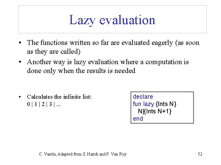
Lazy evaluation • The functions written so far are evaluated eagerly (as soon as they are called) • Another way is lazy evaluation where a computation is done only when the results is needed • Calculates the infinite list: 0 | 1 | 2 | 3 |. . . C. Varela; Adapted from S. Haridi and P. Van Roy declare fun lazy {Ints N} N|{Ints N+1} end 52

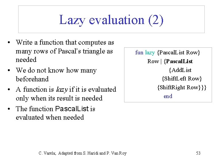
Lazy evaluation (2) • Write a function that computes as many rows of Pascal’s triangle as needed • We do not know how many beforehand • A function is lazy if it is evaluated only when its result is needed • The function Pascal. List is evaluated when needed C. Varela; Adapted from S. Haridi and P. Van Roy fun lazy {Pascal. List Row} Row | {Pascal. List {Add. List {Shift. Left Row} {Shift. Right Row}}} end 53

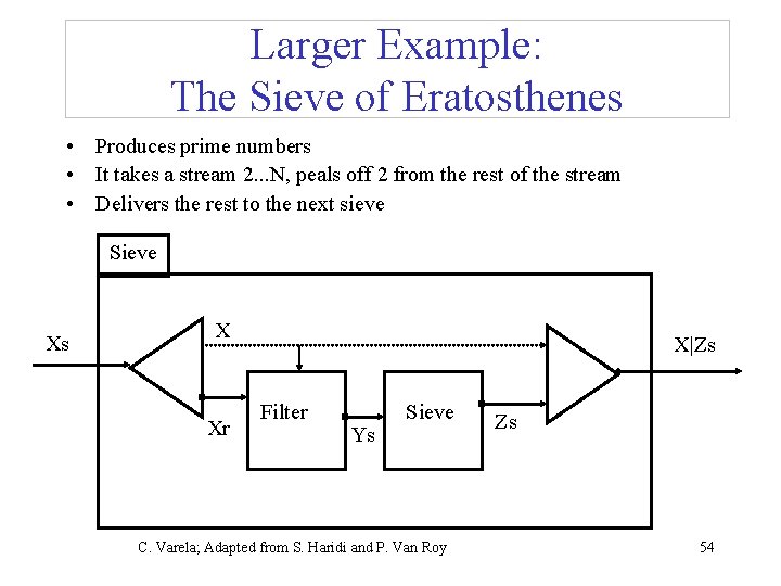
Larger Example: The Sieve of Eratosthenes • Produces prime numbers • It takes a stream 2. . . N, peals off 2 from the rest of the stream • Delivers the rest to the next sieve Sieve Xs X Xr X|Zs Filter Ys Sieve C. Varela; Adapted from S. Haridi and P. Van Roy Zs 54

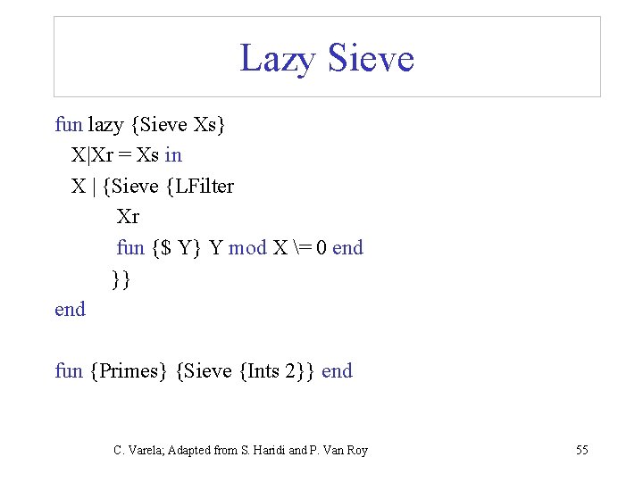
Lazy Sieve fun lazy {Sieve Xs} X|Xr = Xs in X | {Sieve {LFilter Xr fun {$ Y} Y mod X = 0 end }} end fun {Primes} {Sieve {Ints 2}} end C. Varela; Adapted from S. Haridi and P. Van Roy 55

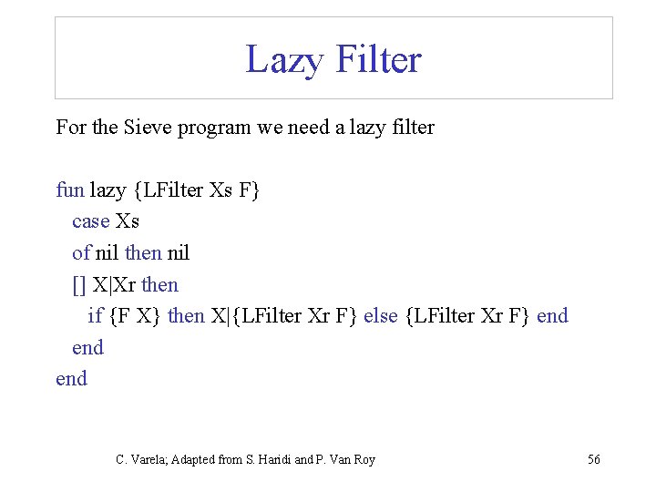
Lazy Filter For the Sieve program we need a lazy filter fun lazy {LFilter Xs F} case Xs of nil then nil [] X|Xr then if {F X} then X|{LFilter Xr F} else {LFilter Xr F} end end C. Varela; Adapted from S. Haridi and P. Van Roy 56

Primes in Haskell ints : : (Num a) => a -> [a] ints n = n : ints (n+1) sieve : : (Integral a) => [a] -> [a] sieve (x: xr) = x: sieve (filter (y -> (y `mod` x /= 0)) xr) primes : : (Integral a) => [a] primes = sieve (ints 2) Functions in Haskell are lazy by default. You can use take 20 primes to get the first 20 elements of the list. C. Varela 57

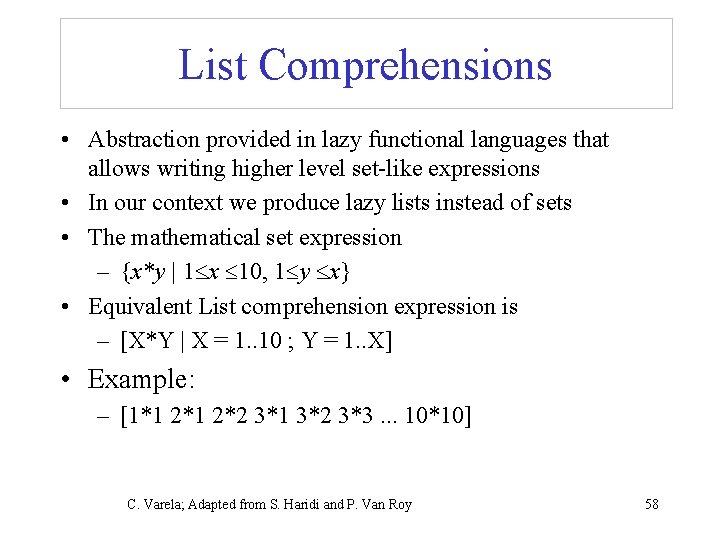
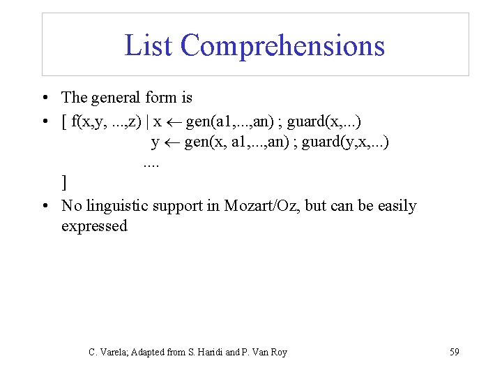
List Comprehensions • Abstraction provided in lazy functional languages that allows writing higher level set-like expressions • In our context we produce lazy lists instead of sets • The mathematical set expression – {x*y | 1 x 10, 1 y x} • Equivalent List comprehension expression is – [X*Y | X = 1. . 10 ; Y = 1. . X] • Example: – [1*1 2*2 3*1 3*2 3*3. . . 10*10] C. Varela; Adapted from S. Haridi and P. Van Roy 58

List Comprehensions • The general form is • [ f(x, y, . . . , z) | x gen(a 1, . . . , an) ; guard(x, . . . ) y gen(x, a 1, . . . , an) ; guard(y, x, . . . ). . ] • No linguistic support in Mozart/Oz, but can be easily expressed C. Varela; Adapted from S. Haridi and P. Van Roy 59

Example 1 • z = [x#x | x from(1, 10)] • Z = {LMap {LFrom 1 10} fun{$ X} X#X end} • z = [x#y | x from(1, 10), y from(1, x)] • Z = {LFlatten {LMap {LFrom 1 10} fun{$ X} {LMap {LFrom 1 X} fun {$ Y} X#Y end } end } } C. Varela; Adapted from S. Haridi and P. Van Roy 60

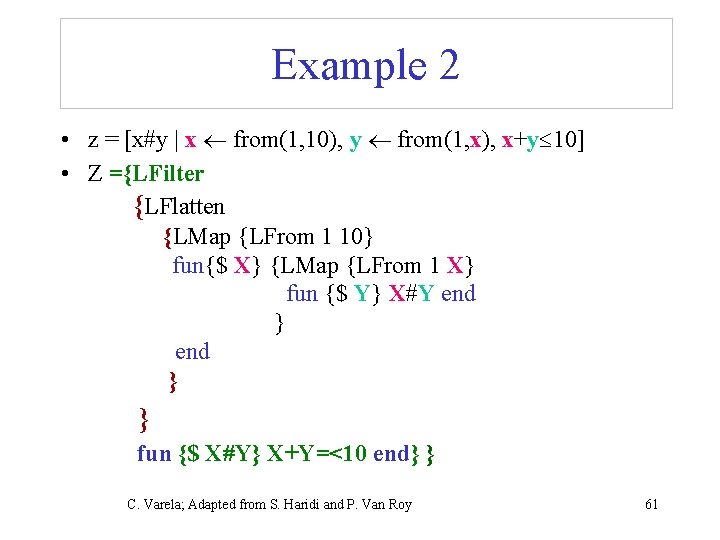
Example 2 • z = [x#y | x from(1, 10), y from(1, x), x+y 10] • Z ={LFilter {LFlatten {LMap {LFrom 1 10} fun{$ X} {LMap {LFrom 1 X} fun {$ Y} X#Y end } end } } fun {$ X#Y} X+Y=<10 end} } C. Varela; Adapted from S. Haridi and P. Van Roy 61

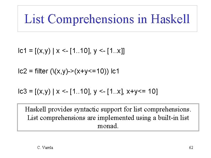
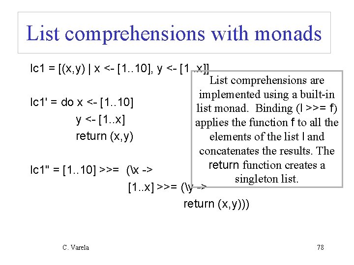
List Comprehensions in Haskell lc 1 = [(x, y) | x <- [1. . 10], y <- [1. . x]] lc 2 = filter ((x, y)->(x+y<=10)) lc 1 lc 3 = [(x, y) | x <- [1. . 10], y <- [1. . x], x+y<= 10] Haskell provides syntactic support for list comprehensions. List comprehensions are implemented using a built-in list monad. C. Varela 62

Quicksort using list comprehensions quicksort : : (Ord a) => [a] -> [a] quicksort [] = [] quicksort (h: t) = quicksort [x | x <- t, x < h] ++ [h] ++ quicksort [x | x <-t, x >= h] C. Varela 63

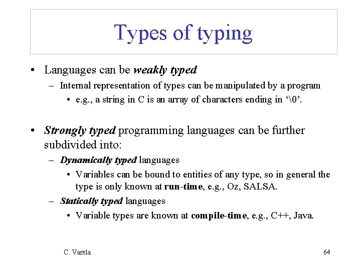
Types of typing • Languages can be weakly typed – Internal representation of types can be manipulated by a program • e. g. , a string in C is an array of characters ending in ‘’. • Strongly typed programming languages can be further subdivided into: – Dynamically typed languages • Variables can be bound to entities of any type, so in general the type is only known at run-time, e. g. , Oz, SALSA. – Statically typed languages • Variable types are known at compile-time, e. g. , C++, Java. C. Varela 64

Type Checking and Inference • Type checking is the process of ensuring a program is welltyped. – One strategy often used is abstract interpretation: • The principle of getting partial information about the answers from partial information about the inputs • Programmer supplies types of variables and type-checker deduces types of other expressions for consistency • Type inference frees programmers from annotating variable types: types are inferred from variable usage, e. g. ML, Haskell. C. Varela 65

Abstract data types • A datatype is a set of values and an associated set of operations • A datatype is abstract only if it is completely described by its set of operations regardless of its implementation • This means that it is possible to change the implementation of the datatype without changing its use • The datatype is thus described by a set of procedures • These operations are the only thing that a user of the abstraction can assume C. Varela; Adapted w/permission from S. Haridi and P. Van Roy 66

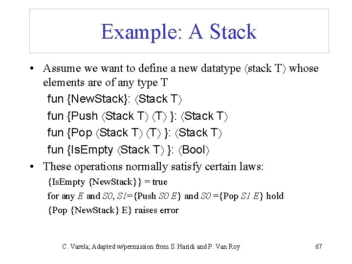
Example: A Stack • Assume we want to define a new datatype stack T whose elements are of any type T fun {New. Stack}: Stack T fun {Push Stack T T }: Stack T fun {Pop Stack T T }: Stack T fun {Is. Empty Stack T }: Bool • These operations normally satisfy certain laws: {Is. Empty {New. Stack}} = true for any E and S 0, S 1={Push S 0 E} and S 0 ={Pop S 1 E} hold {Pop {New. Stack} E} raises error C. Varela; Adapted w/permission from S. Haridi and P. Van Roy 67

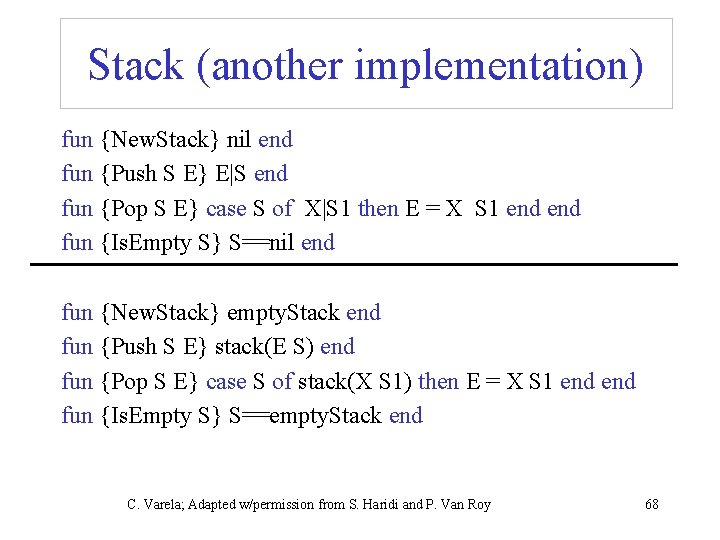
Stack (another implementation) fun {New. Stack} nil end fun {Push S E} E|S end fun {Pop S E} case S of X|S 1 then E = X S 1 end fun {Is. Empty S} S==nil end fun {New. Stack} empty. Stack end fun {Push S E} stack(E S) end fun {Pop S E} case S of stack(X S 1) then E = X S 1 end fun {Is. Empty S} S==empty. Stack end C. Varela; Adapted w/permission from S. Haridi and P. Van Roy 68

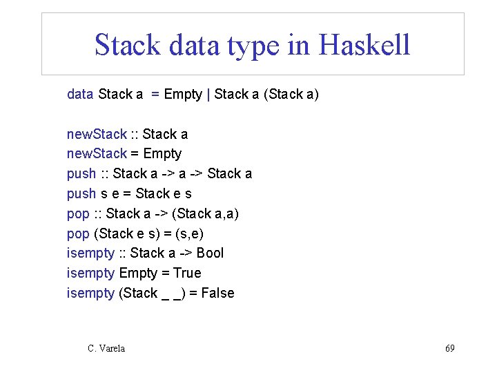
Stack data type in Haskell data Stack a = Empty | Stack a (Stack a) new. Stack : : Stack a new. Stack = Empty push : : Stack a -> Stack a push s e = Stack e s pop : : Stack a -> (Stack a, a) pop (Stack e s) = (s, e) isempty : : Stack a -> Bool isempty Empty = True isempty (Stack _ _) = False C. Varela 69

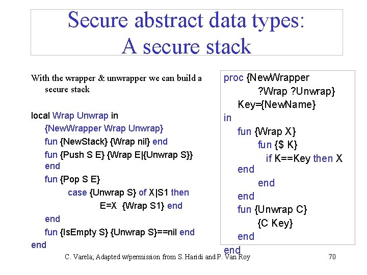
Secure abstract data types: A secure stack With the wrapper & unwrapper we can build a secure stack local Wrap Unwrap in {New. Wrapper Wrap Unwrap} fun {New. Stack} {Wrap nil} end fun {Push S E} {Wrap E|{Unwrap S}} end fun {Pop S E} case {Unwrap S} of X|S 1 then E=X {Wrap S 1} end fun {Is. Empty S} {Unwrap S}==nil end proc {New. Wrapper ? Wrap ? Unwrap} Key={New. Name} in fun {Wrap X} fun {$ K} if K==Key then X end end fun {Unwrap C} {C Key} end C. Varela; Adapted w/permission from S. Haridi and P. Van Roy 70

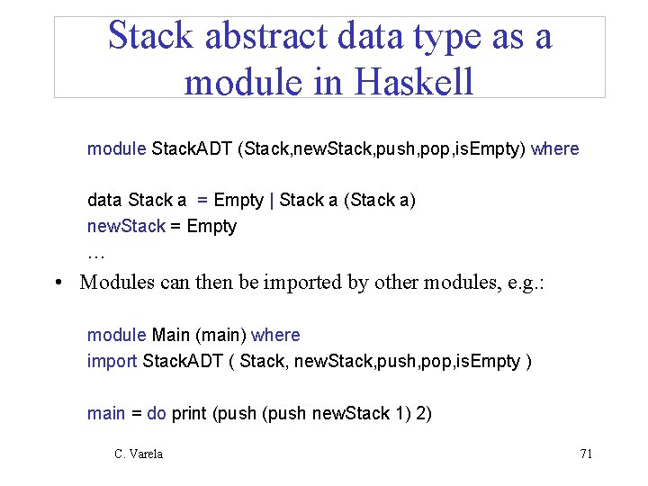
Stack abstract data type as a module in Haskell module Stack. ADT (Stack, new. Stack, push, pop, is. Empty) where data Stack a = Empty | Stack a (Stack a) new. Stack = Empty … • Modules can then be imported by other modules, e. g. : module Main (main) where import Stack. ADT ( Stack, new. Stack, push, pop, is. Empty ) main = do print (push new. Stack 1) 2) C. Varela 71

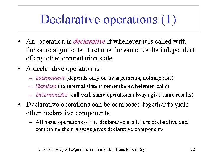
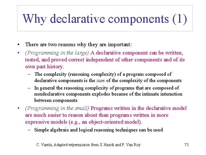
Declarative operations (1) • An operation is declarative if whenever it is called with the same arguments, it returns the same results independent of any other computation state • A declarative operation is: – Independent (depends only on its arguments, nothing else) – Stateless (no internal state is remembered between calls) – Deterministic (call with same operations always give same results) • Declarative operations can be composed together to yield other declarative components – All basic operations of the declarative model are declarative and combining them always gives declarative components C. Varela; Adapted w/permission from S. Haridi and P. Van Roy 72

Why declarative components (1) • There are two reasons why they are important: • (Programming in the large) A declarative component can be written, tested, and proved correct independent of other components and of its own past history. – The complexity (reasoning complexity) of a program composed of declarative components is the sum of the complexity of the components – In general the reasoning complexity of programs that are composed of nondeclarative components explodes because of the intimate interaction between components • (Programming in the small) Programs written in the declarative model are much easier to reason about than programs written in more expressive models (e. g. , an object-oriented model). – Simple algebraic and logical reasoning techniques can be used C. Varela; Adapted w/permission from S. Haridi and P. Van Roy 73

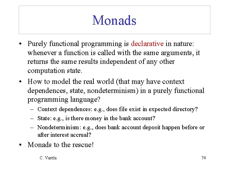
Monads • Purely functional programming is declarative in nature: whenever a function is called with the same arguments, it returns the same results independent of any other computation state. • How to model the real world (that may have context dependences, state, nondeterminism) in a purely functional programming language? – Context dependences: e. g. , does file exist in expected directory? – State: e. g. , is there money in the bank account? – Nondeterminism: e. g. , does bank account deposit happen before or after interest accrual? • Monads to the rescue! C. Varela 74

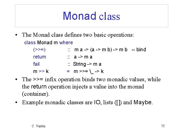
Monad class • The Monad class defines two basic operations: class Monad m where (>>=) : : m a -> (a -> m b) -> m b -- bind return : : a -> m a fail : : String -> m a m >> k = m >>= _ -> k • The >>= infix operation binds two monadic values, while the return operation injects a value into the monad (container). • Example monadic classes are IO, lists ([]) and Maybe. C. Varela 75

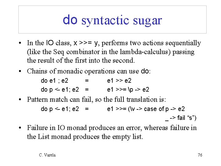
do syntactic sugar • In the IO class, x >>= y, performs two actions sequentially (like the Seq combinator in the lambda-calculus) passing the result of the first into the second. • Chains of monadic operations can use do: do e 1 ; e 2 do p <- e 1; e 2 = = e 1 >> e 2 e 1 >>= p -> e 2 • Pattern match can fail, so the full translation is: do p <- e 1; e 2 = e 1 >>= (v -> case of p -> e 2 _ -> fail “s”) • Failure in IO monad produces an error, whereas failure in the List monad produces the empty list. C. Varela 76

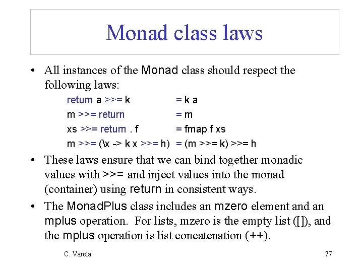
Monad class laws • All instances of the Monad class should respect the following laws: return a >>= k m >>= return xs >>= return. f m >>= (x -> k x >>= h) =ka =m = fmap f xs = (m >>= k) >>= h • These laws ensure that we can bind together monadic values with >>= and inject values into the monad (container) using return in consistent ways. • The Monad. Plus class includes an mzero element and an mplus operation. For lists, mzero is the empty list ([]), and the mplus operation is list concatenation (++). C. Varela 77

List comprehensions with monads lc 1 = [(x, y) | x <- [1. . 10], y <- [1. . x]] List comprehensions are implemented using a built-in lc 1' = do x <- [1. . 10] list monad. Binding (l >>= f) y <- [1. . x] applies the function f to all the return (x, y) elements of the list l and concatenates the results. The return function creates a lc 1'' = [1. . 10] >>= (x -> singleton list. [1. . x] >>= (y -> return (x, y))) C. Varela 78

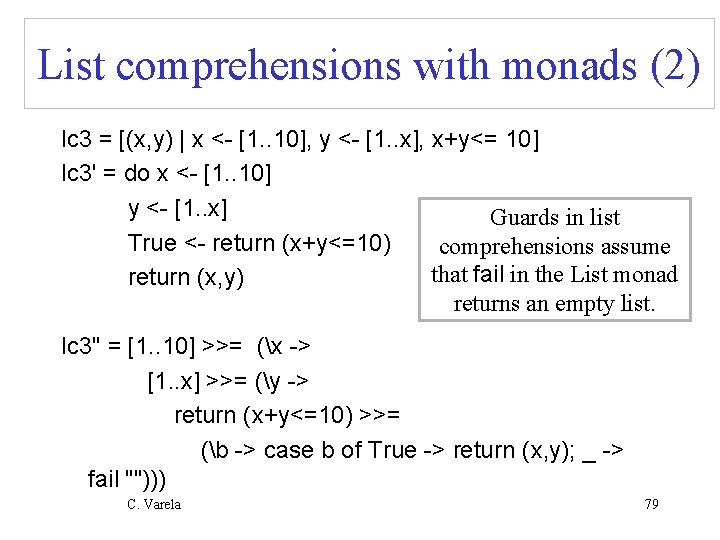
List comprehensions with monads (2) lc 3 = [(x, y) | x <- [1. . 10], y <- [1. . x], x+y<= 10] lc 3' = do x <- [1. . 10] y <- [1. . x] Guards in list True <- return (x+y<=10) comprehensions assume that fail in the List monad return (x, y) returns an empty list. lc 3'' = [1. . 10] >>= (x -> [1. . x] >>= (y -> return (x+y<=10) >>= (b -> case b of True -> return (x, y); _ -> fail ""))) C. Varela 79

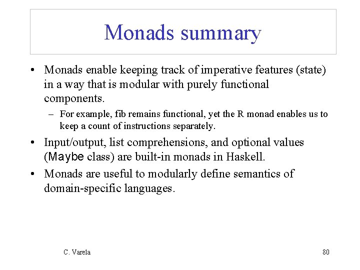
Monads summary • Monads enable keeping track of imperative features (state) in a way that is modular with purely functional components. – For example, fib remains functional, yet the R monad enables us to keep a count of instructions separately. • Input/output, list comprehensions, and optional values (Maybe class) are built-in monads in Haskell. • Monads are useful to modularly define semantics of domain-specific languages. C. Varela 80