Programming in R InputOutput Statistics and Graphics Programming

Programming in R Input/Output, Statistics and Graphics Programming in R

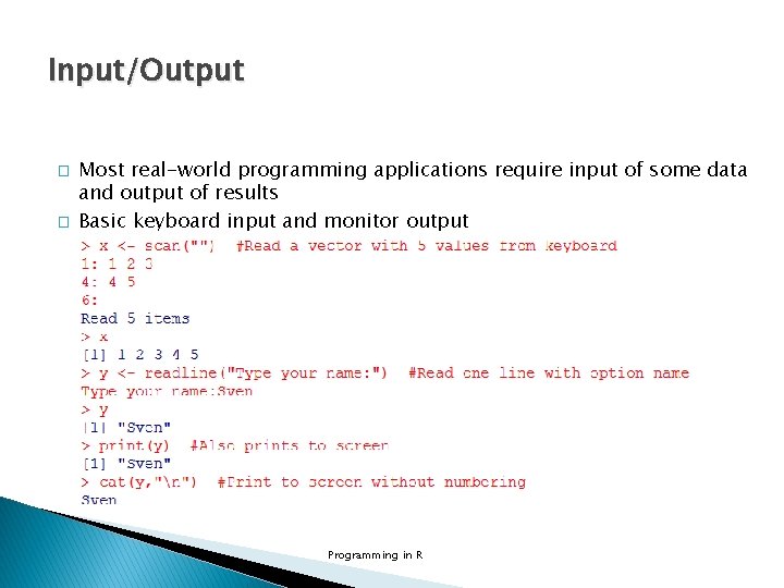
Input/Output � � Most real-world programming applications require input of some data and output of results Basic keyboard input and monitor output Programming in R

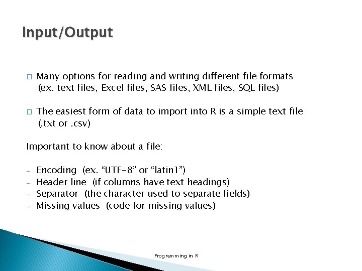
Input/Output � � Many options for reading and writing different file formats (ex. text files, Excel files, SAS files, XML files, SQL files) The easiest form of data to import into R is a simple text file (. txt or. csv) Important to know about a file: - Encoding (ex. “UTF-8” or “latin 1”) Header line (if columns have text headings) Separator (the character used to separate fields) Missing values (code for missing values) Programming in R

Input/Output � scan() is an elaborate function that can be used to read data from various file types and sites, and it also provides the basis for more convenient functions like read. table() and read. csv() mat. txt in working directory Programming in R

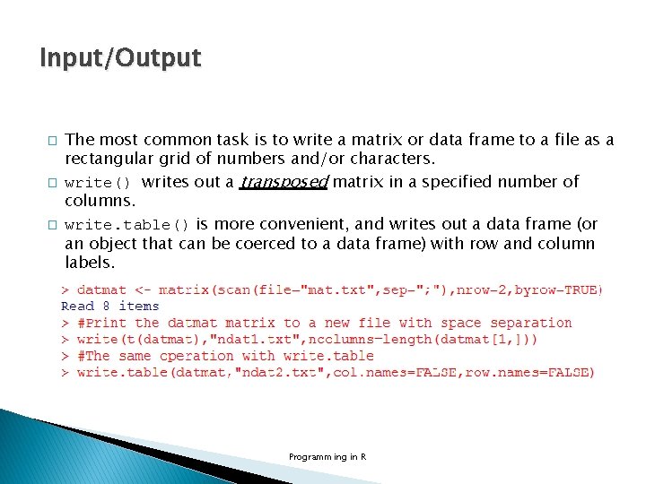
Input/Output � � � The most common task is to write a matrix or data frame to a file as a rectangular grid of numbers and/or characters. write() writes out a transposed matrix in a specified number of columns. write. table() is more convenient, and writes out a data frame (or an object that can be coerced to a data frame) with row and column labels. Programming in R

Input/Output � Connections in R provides another way of reading and writing files. It is based on opening of a connection (file() or url()), reading some data (ex. read. Lines(), scan()) and/or writing some results (ex. write. Lines(), cat()) and finally closing the connection (close()) mat. txt in working directory Programming in R

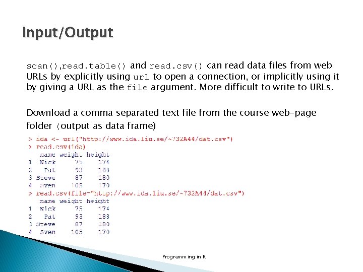
Input/Output scan(), read. table() and read. csv() can read data files from web URLs by explicitly using url to open a connection, or implicitly using it by giving a URL as the file argument. More difficult to write to URLs. Download a comma separated text file from the course web-page folder (output as data frame) Programming in R

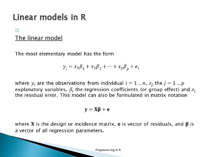
Linear models in R � Programming in R

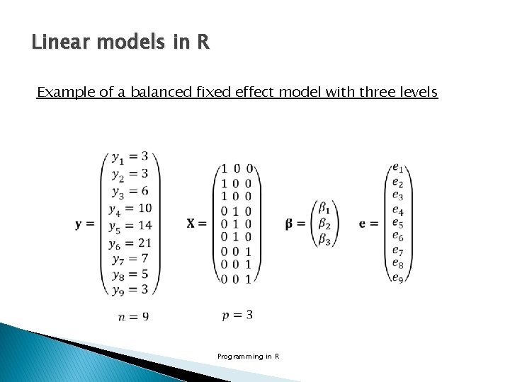
Linear models in R Example of a balanced fixed effect model with three levels Programming in R

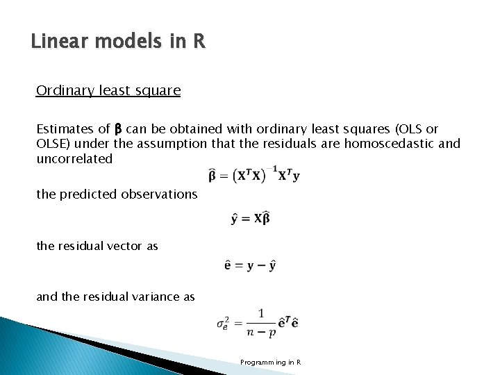
Linear models in R Ordinary least square Estimates of β can be obtained with ordinary least squares (OLS or OLSE) under the assumption that the residuals are homoscedastic and uncorrelated the predicted observations the residual vector as and the residual variance as Programming in R

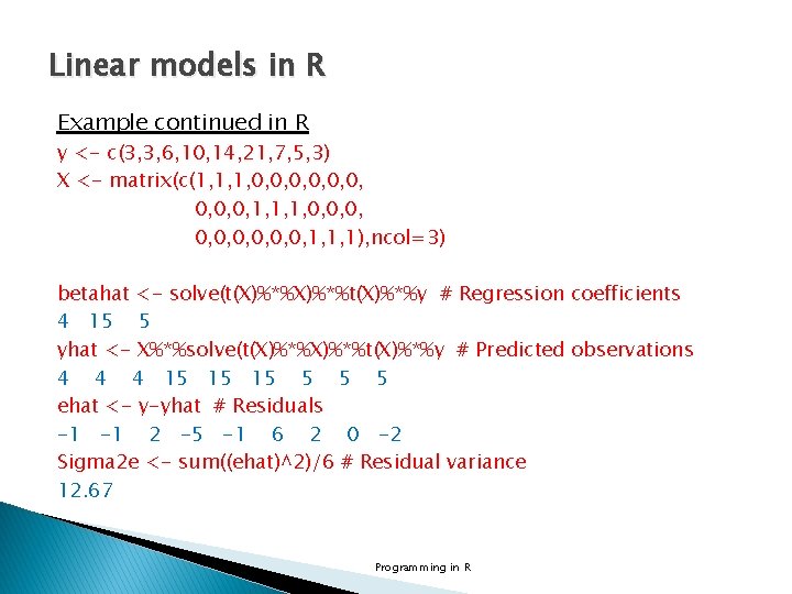
Linear models in R Example continued in R y <- c(3, 3, 6, 10, 14, 21, 7, 5, 3) X <- matrix(c(1, 1, 1, 0, 0, 0, 0, 0, 1, 1, 1), ncol=3) betahat <- solve(t(X)%*%t(X)%*%y # Regression coefficients 4 15 5 yhat <- X%*%solve(t(X)%*%t(X)%*%y # Predicted observations 4 4 4 15 15 15 5 ehat <- y-yhat # Residuals -1 -1 2 -5 -1 6 2 0 -2 Sigma 2 e <- sum((ehat)^2)/6 # Residual variance 12. 67 Programming in R

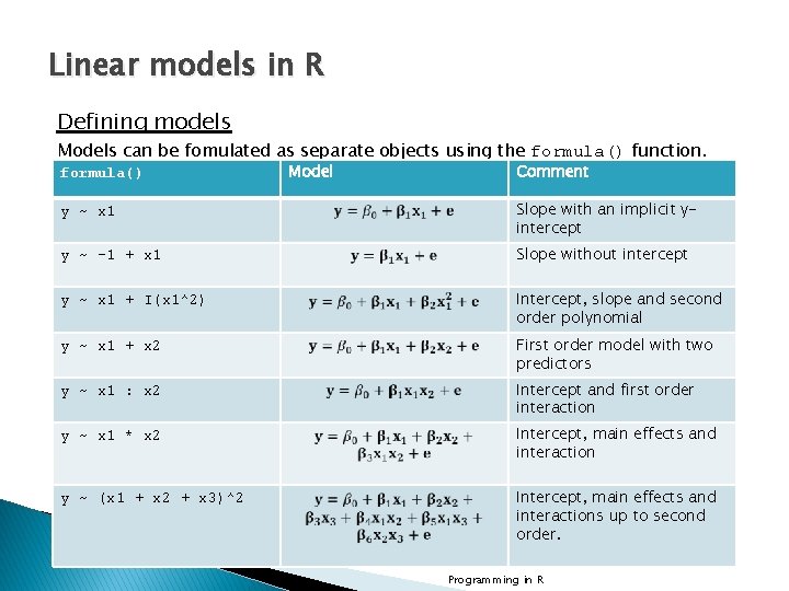
Linear models in R Defining models Models can be fomulated as separate objects using the formula() function. formula() Model Comment y ~ x 1 Slope with an implicit yintercept y ~ -1 + x 1 Slope without intercept y ~ x 1 + I(x 1^2) Intercept, slope and second order polynomial y ~ x 1 + x 2 First order model with two predictors y ~ x 1 : x 2 Intercept and first order interaction y ~ x 1 * x 2 Intercept, main effects and interaction y ~ (x 1 + x 2 + x 3)^2 Intercept, main effects and interactions up to second order. Programming in R

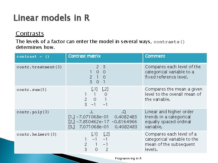
Linear models in R Contrasts The levels of a factor can enter the model in several ways, contrasts() determines how. contrast = () contr. treatment(3) contr. sum(3) contr. poly(3) contr. helmert(3) Contrast matrix 2 1 0 2 1 3 0 Comment 3 0 0 1 Compares each level of the categorical variable to a fixed reference level. [, 1] [, 2] 1 1 0 2 0 1 3 -1 -1 Compares the mean a given level to the overall mean of the variable. . L. Q [1, ] -7. 071068 e-01 0. 4082483 [2, ] -7. 850462 e-17 -0. 8164966 [3, ] 7. 071068 e-01 0. 4082483 [, 1] 1 -1 2 1 3 0 [, 2] -1 -1 2 Linear and higher order trends in a categorical equally spaced ordinal variable. Compares each level of a categorical variable to the mean of the subsequent levels. Programming in R

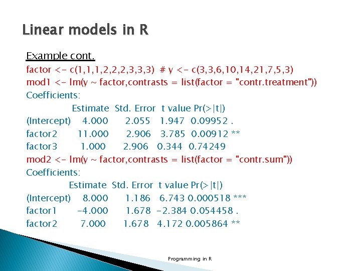
Linear models in R Example cont. factor <- c(1, 1, 1, 2, 2, 2, 3, 3, 3) # y <- c(3, 3, 6, 10, 14, 21, 7, 5, 3) mod 1 <- lm(y ~ factor, contrasts = list(factor = "contr. treatment")) Coefficients: Estimate Std. Error t value Pr(>|t|) (Intercept) 4. 000 2. 055 1. 947 0. 09952. factor 2 11. 000 2. 906 3. 785 0. 00912 ** factor 3 1. 000 2. 906 0. 344 0. 74249 mod 2 <- lm(y ~ factor, contrasts = list(factor = "contr. sum")) Coefficients: Estimate Std. Error t value Pr(>|t|) (Intercept) 8. 000 1. 186 6. 743 0. 000518 *** factor 1 -4. 000 1. 678 -2. 384 0. 054458. factor 2 7. 000 1. 678 4. 172 0. 005864 ** Programming in R

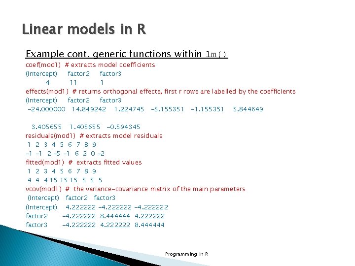
Linear models in R Example cont. generic functions within lm() coef(mod 1) # extracts model coefficients (Intercept) factor 2 factor 3 4 11 1 effects(mod 1) # returns orthogonal effects, first r rows are labelled by the coefficients (Intercept) factor 2 factor 3 -24. 000000 14. 849242 1. 224745 -5. 155351 -1. 155351 5. 844649 3. 405655 1. 405655 -0. 594345 residuals(mod 1) # extracts model residuals 1 2 3 4 5 6 7 8 9 -1 -1 2 -5 -1 6 2 0 -2 fitted(mod 1) # extracts fitted values 1 2 3 4 5 6 7 8 9 4 4 4 15 15 15 5 vcov(mod 1) # the variance-covariance matrix of the main parameters (Intercept) factor 2 factor 3 (Intercept) 4. 222222 -4. 222222 factor 2 -4. 222222 8. 444444 4. 222222 factor 3 -4. 222222 8. 444444 Programming in R

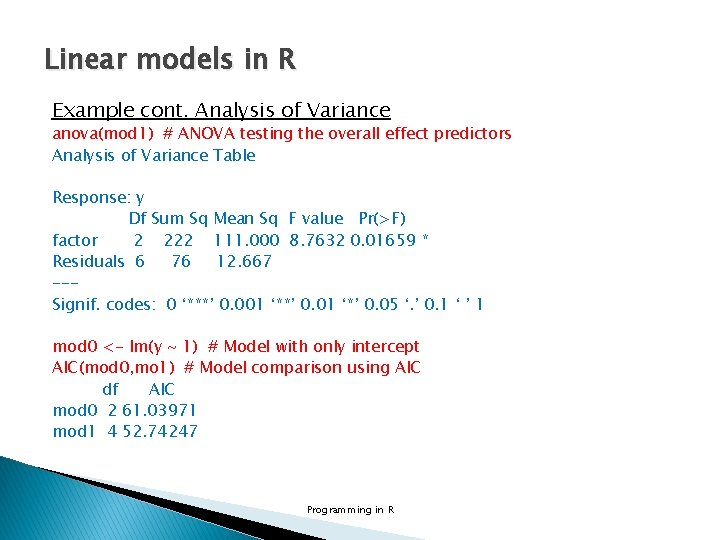
Linear models in R Example cont. Analysis of Variance anova(mod 1) # ANOVA testing the overall effect predictors Analysis of Variance Table Response: y Df Sum Sq Mean Sq F value Pr(>F) factor 2 222 111. 000 8. 7632 0. 01659 * Residuals 6 76 12. 667 --Signif. codes: 0 ‘***’ 0. 001 ‘**’ 0. 01 ‘*’ 0. 05 ‘. ’ 0. 1 ‘ ’ 1 mod 0 <- lm(y ~ 1) # Model with only intercept AIC(mod 0, mo 1) # Model comparison using AIC df AIC mod 0 2 61. 03971 mod 1 4 52. 74247 Programming in R

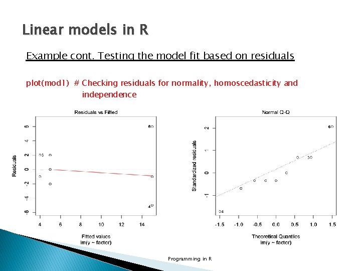
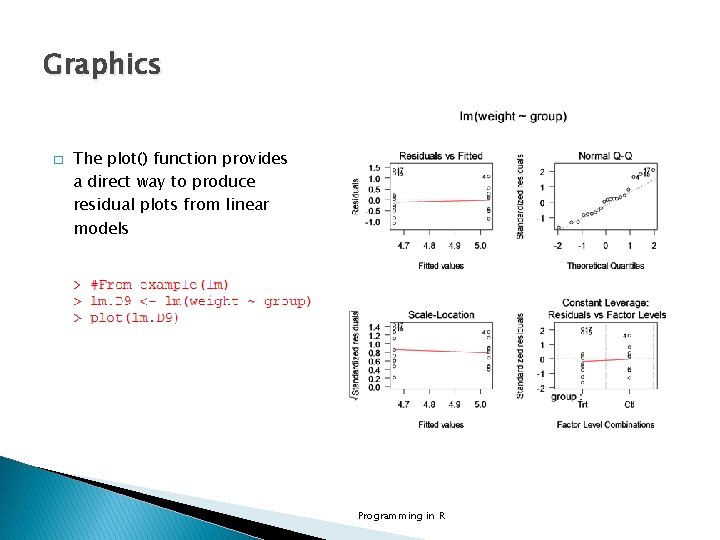
Linear models in R Example cont. Testing the model fit based on residuals plot(mod 1) # Checking residuals for normality, homoscedasticity and independence Programming in R

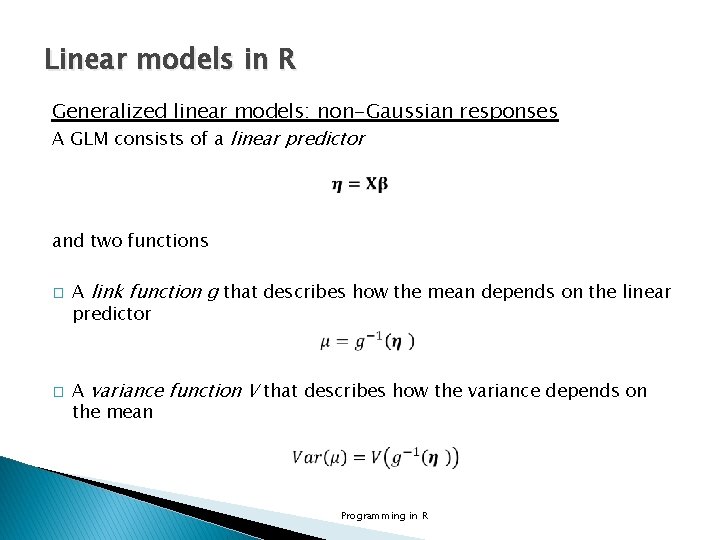
Linear models in R Generalized linear models: non-Gaussian responses A GLM consists of a linear predictor and two functions � � A link function g that describes how the mean depends on the linear predictor A variance function V that describes how the variance depends on the mean Programming in R

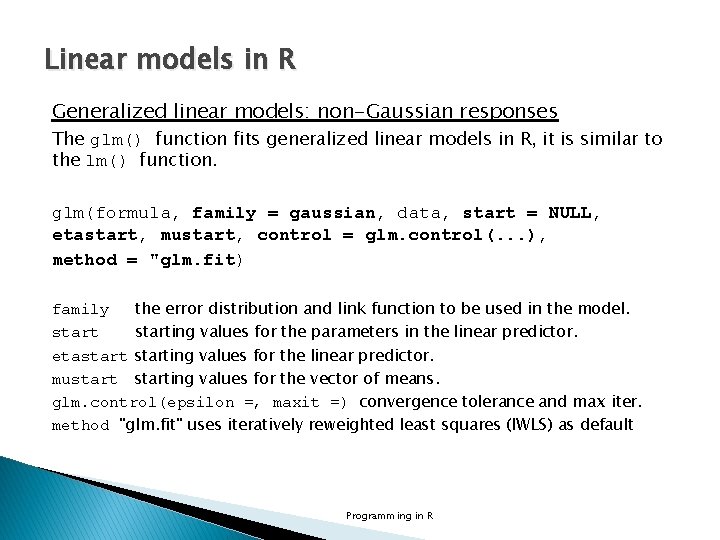
Linear models in R Generalized linear models: non-Gaussian responses The glm() function fits generalized linear models in R, it is similar to the lm() function. glm(formula, family = gaussian, data, start = NULL, etastart, mustart, control = glm. control(. . . ), method = "glm. fit) family the error distribution and link function to be used in the model. starting values for the parameters in the linear predictor. etastarting values for the linear predictor. mustarting values for the vector of means. glm. control(epsilon =, maxit =) convergence tolerance and max iter. method "glm. fit" uses iteratively reweighted least squares (IWLS) as default Programming in R

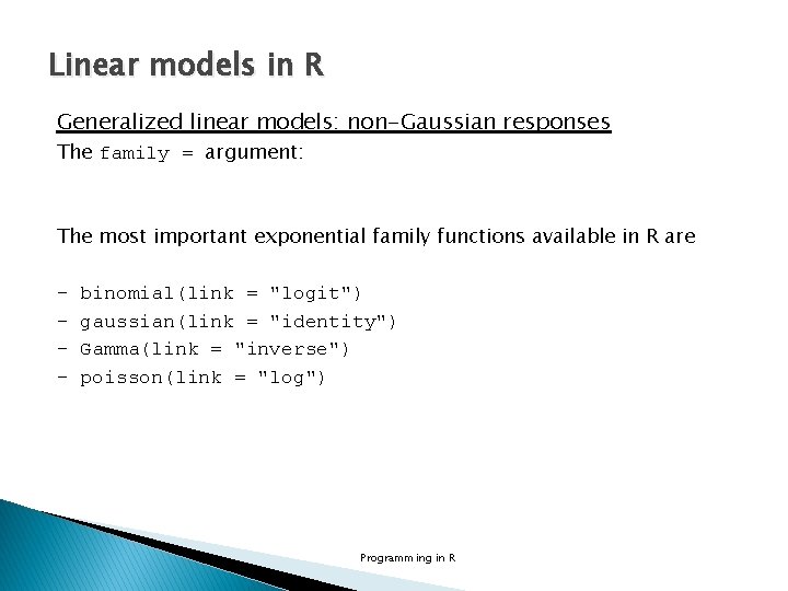
Linear models in R Generalized linear models: non-Gaussian responses The family = argument: The most important exponential family functions available in R are - binomial(link = "logit") gaussian(link = "identity") Gamma(link = "inverse") poisson(link = "log") Programming in R

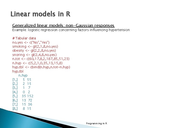
Linear models in R Generalized linear models: non-Gaussian responses Example: logistic regression concerning factors influencing hypertension # Tabular data no. yes <- c("No", "Yes") smoking <- gl(2, 1, 8, no. yes) obesity <- gl(2, 2, 8, no. yes) snoring <- gl(2, 4, 8, no. yes) n. tot <- c(60, 17, 8, 2, 187, 85, 51, 23) n. hyp <- c(5, 2, 1, 0, 35, 13, 15, 8) hyp. tbl <- cbind(n. hyp, n. tot-n. hyp) hyp. tbl n. hyp [1, ] 5 55 [2, ] 2 15 [3, ] 1 7 [4, ] 0 2 [5, ] 35 152 [6, ] 13 72 [7, ] 15 36 [8, ] 8 15 Programming in R

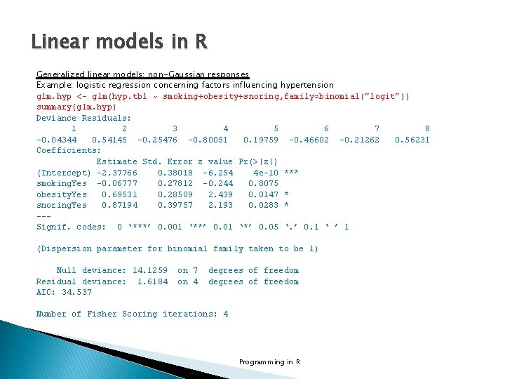
Linear models in R Generalized linear models: non-Gaussian responses Example: logistic regression concerning factors influencing hypertension glm. hyp <- glm(hyp. tbl ~ smoking+obesity+snoring, family=binomial("logit")) summary(glm. hyp) Deviance Residuals: 1 2 3 4 5 6 7 8 -0. 04344 0. 54145 -0. 25476 -0. 80051 0. 19759 -0. 46602 -0. 21262 0. 56231 Coefficients: Estimate Std. Error z value Pr(>|z|) (Intercept) -2. 37766 0. 38018 -6. 254 4 e-10 *** smoking. Yes -0. 06777 0. 27812 -0. 244 0. 8075 obesity. Yes 0. 69531 0. 28509 2. 439 0. 0147 * snoring. Yes 0. 87194 0. 39757 2. 193 0. 0283 * --Signif. codes: 0 ‘***’ 0. 001 ‘**’ 0. 01 ‘*’ 0. 05 ‘. ’ 0. 1 ‘ ’ 1 (Dispersion parameter for binomial family taken to be 1) Null deviance: 14. 1259 Residual deviance: 1. 6184 AIC: 34. 537 on 4 degrees of freedom Number of Fisher Scoring iterations: 4 Programming in R

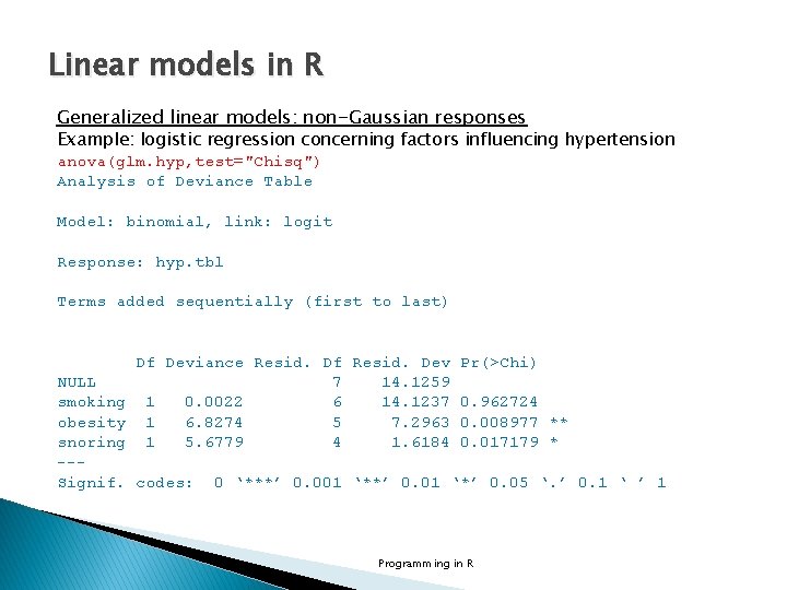
Linear models in R Generalized linear models: non-Gaussian responses Example: logistic regression concerning factors influencing hypertension anova(glm. hyp, test="Chisq") Analysis of Deviance Table Model: binomial, link: logit Response: hyp. tbl Terms added sequentially (first to last) Df Deviance Resid. Df Resid. Dev Pr(>Chi) NULL 7 14. 1259 smoking 1 0. 0022 6 14. 1237 0. 962724 obesity 1 6. 8274 5 7. 2963 0. 008977 ** snoring 1 5. 6779 4 1. 6184 0. 017179 * --Signif. codes: 0 ‘***’ 0. 001 ‘**’ 0. 01 ‘*’ 0. 05 ‘. ’ 0. 1 ‘ ’ 1 Programming in R

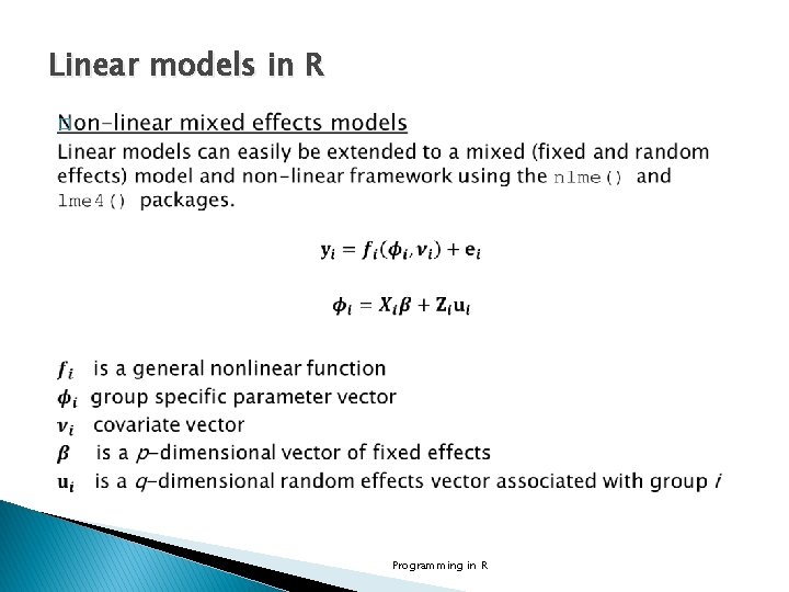
Linear models in R � Programming in R

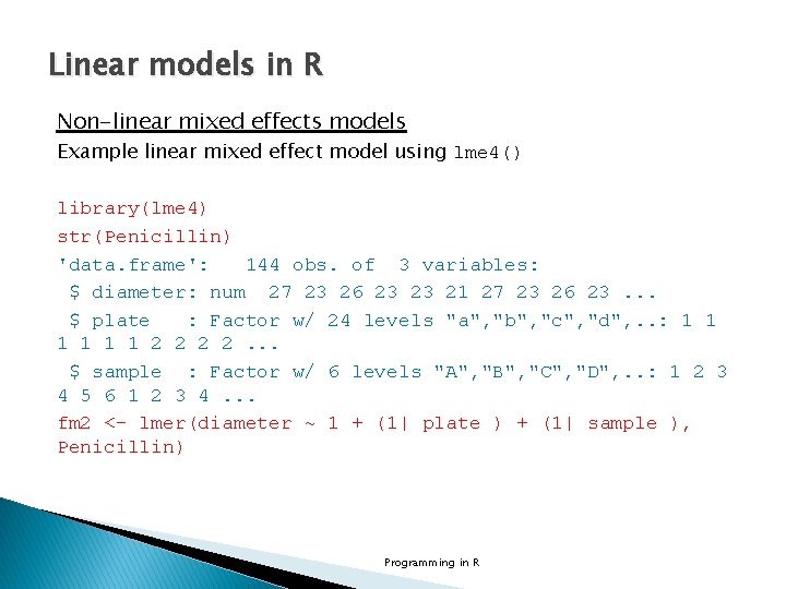
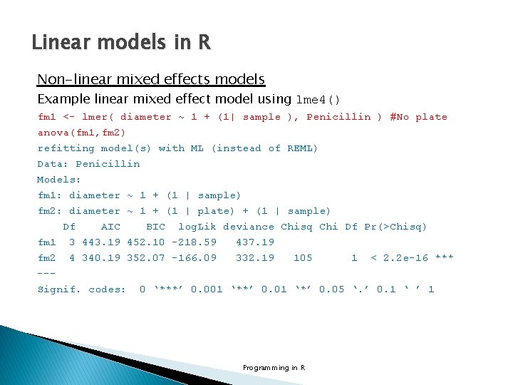
Linear models in R Non-linear mixed effects models Example linear mixed effect model using lme 4() library(lme 4) str(Penicillin) 'data. frame': 144 obs. of 3 variables: $ diameter: num 27 23 26 23 23 21 27 23 26 23. . . $ plate : Factor w/ 24 levels "a", "b", "c", "d", . . : 1 1 1 2 2. . . $ sample : Factor w/ 6 levels "A", "B", "C", "D", . . : 1 2 3 4 5 6 1 2 3 4. . . fm 2 <- lmer(diameter ~ 1 + (1| plate ) + (1| sample ), Penicillin) Programming in R

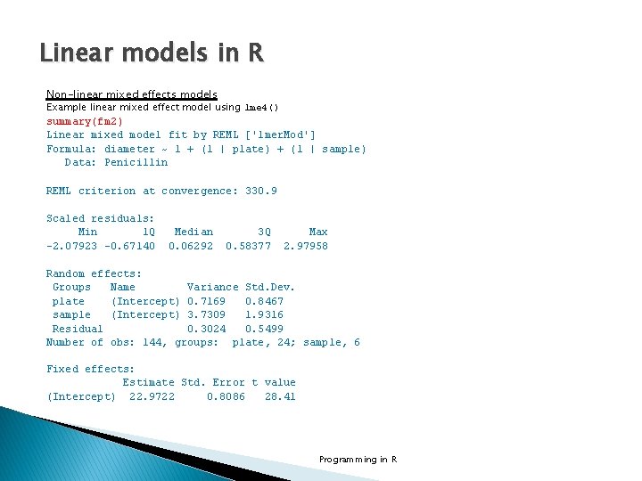
Linear models in R Non-linear mixed effects models Example linear mixed effect model using lme 4() summary(fm 2) Linear mixed model fit by REML ['lmer. Mod'] Formula: diameter ~ 1 + (1 | plate) + (1 | sample) Data: Penicillin REML criterion at convergence: 330. 9 Scaled residuals: Min 1 Q -2. 07923 -0. 67140 Median 0. 06292 3 Q 0. 58377 Max 2. 97958 Random effects: Groups Name Variance Std. Dev. plate (Intercept) 0. 7169 0. 8467 sample (Intercept) 3. 7309 1. 9316 Residual 0. 3024 0. 5499 Number of obs: 144, groups: plate, 24; sample, 6 Fixed effects: Estimate Std. Error t value (Intercept) 22. 9722 0. 8086 28. 41 Programming in R

Linear models in R Non-linear mixed effects models Example linear mixed effect model using lme 4() fm 1 <- lmer( diameter ~ 1 + (1| sample ), Penicillin ) #No plate anova(fm 1, fm 2) refitting model(s) with ML (instead of REML) Data: Penicillin Models: fm 1: diameter ~ 1 + (1 | sample) fm 2: diameter ~ 1 + (1 | plate) + (1 | sample) Df AIC BIC log. Lik deviance Chisq Chi Df Pr(>Chisq) fm 1 3 443. 19 452. 10 -218. 59 437. 19 fm 2 4 340. 19 352. 07 -166. 09 332. 19 105 1 < 2. 2 e-16 *** --Signif. codes: 0 ‘***’ 0. 001 ‘**’ 0. 01 ‘*’ 0. 05 ‘. ’ 0. 1 ‘ ’ 1 Programming in R

Graphics � R has advanced graphics capabilities. Functions in the graphics systems and graphics packages can be broken down into three main types: 1. high-level functions that produce complete plots 2. low-level functions that add further output to an existing plot 3. functions for working interactively with graphical output. � � The traditional system provides the majority of the high-level functions currently available in R. The grid system offers a much wider range of possibilities and better support for combination with other output (for example interactive plots). The lattice package is based on the grid system. Programming in R

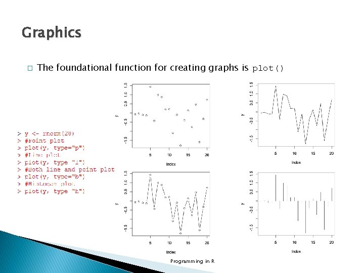
Graphics � The foundational function for creating graphs is plot() Programming in R

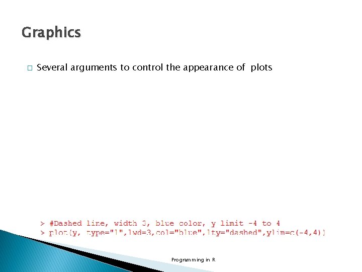
Graphics � Several arguments to control the appearance of plots Programming in R

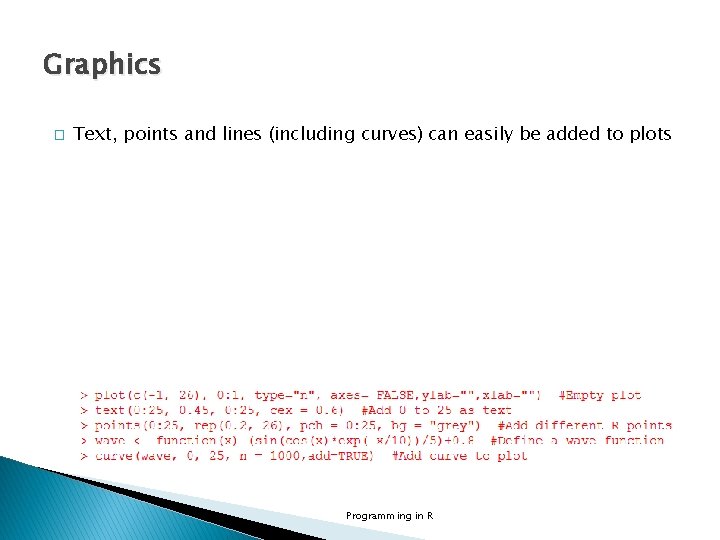
Graphics � Text, points and lines (including curves) can easily be added to plots Programming in R

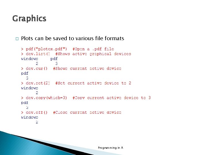
Graphics � Plots can be saved to various file formats Programming in R

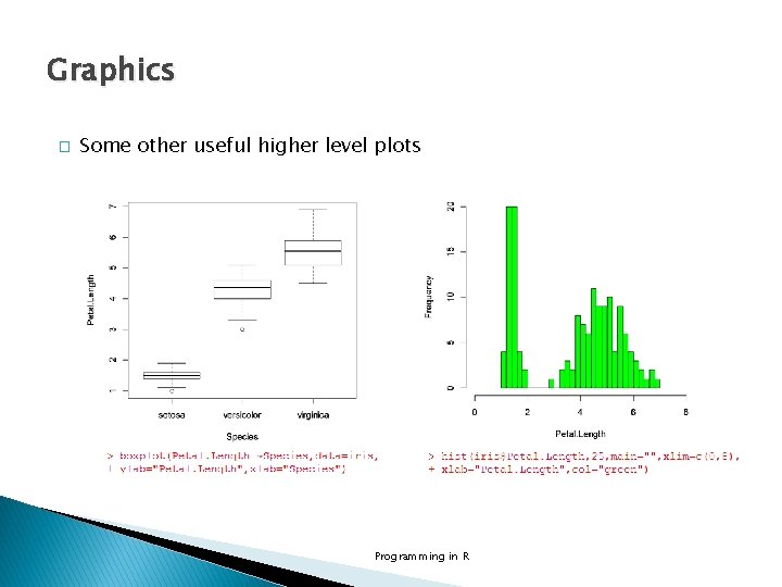
Graphics � Some other useful higher level plots Programming in R

Graphics � The plot() function provides a direct way to produce residual plots from linear models Programming in R

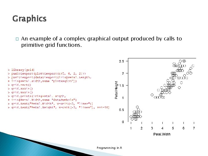
Graphics � � � The grid graphics system provides no high-level plotting functions itself, but there are several advantages to producing a plot using the grid system, including greater flexibility in adding further output to the plot, and the ability to interactively edit the plot. There are grid functions to draw primitive graphical output such as lines, text, and polygons, plus some slightly higher-level graphical components such as axes. Complex graphical output is produced by making a sequence of calls to these lower-level functions. The grid and lattice packages provide both lower and high level functions based on the grid system. Programming in R

Graphics � An example of a complex graphical output produced by calls to primitive grid functions. Programming in R

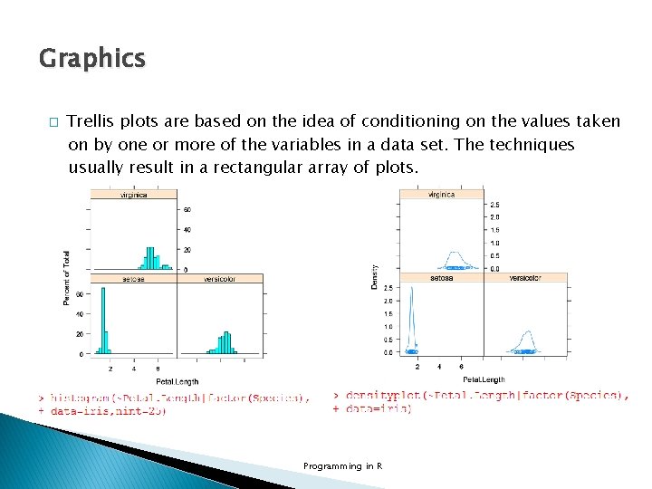
Graphics � The lattice package is a powerful and elegant high-level data visualization system, with an emphasis on multivariate data. It uses the grid package and can be considered an implementation of the general principles of Trellis graphics. Programming in R

Graphics � Trellis plots are based on the idea of conditioning on the values taken on by one or more of the variables in a data set. The techniques usually result in a rectangular array of plots. Programming in R

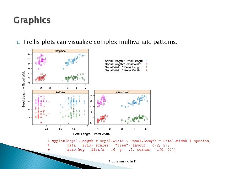
Graphics � Trellis plots can visualize complex multivariate patterns. Programming in R

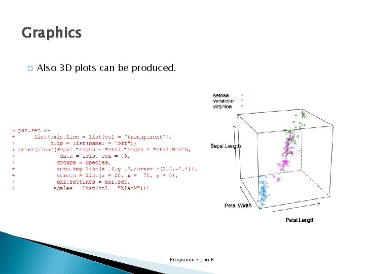
Graphics � Also 3 D plots can be produced. Programming in R

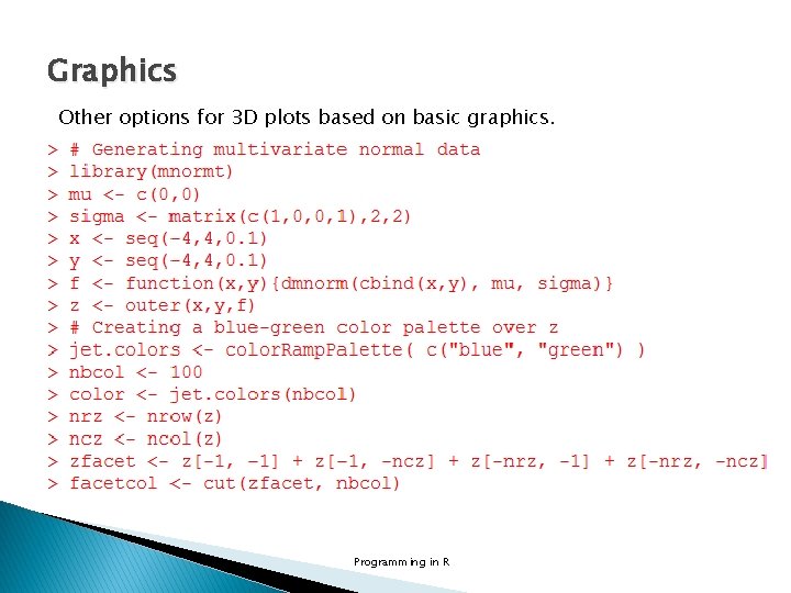
Graphics Other options for 3 D plots based on basic graphics. Programming in R

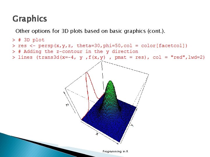
Graphics Other options for 3 D plots based on basic graphics (cont. ). Programming in R