PROGRAMMING IN HASKELL Chapter 15 Lazy Evaluation 0

PROGRAMMING IN HASKELL Chapter 15 – Lazy Evaluation 0

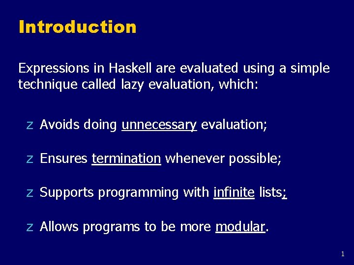
Introduction Expressions in Haskell are evaluated using a simple technique called lazy evaluation, which: z Avoids doing unnecessary evaluation; z Ensures termination whenever possible; z Supports programming with infinite lists; z Allows programs to be more modular. 1

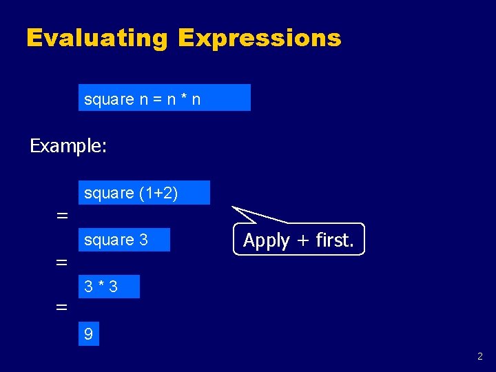
Evaluating Expressions square n = n * n Example: square (1+2) = square 3 = = Apply + first. 3*3 9 2

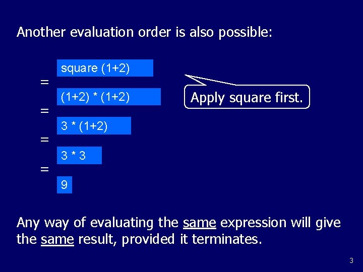
Another evaluation order is also possible: = = square (1+2) * (1+2) Apply square first. 3 * (1+2) 3*3 9 Any way of evaluating the same expression will give the same result, provided it terminates. 3

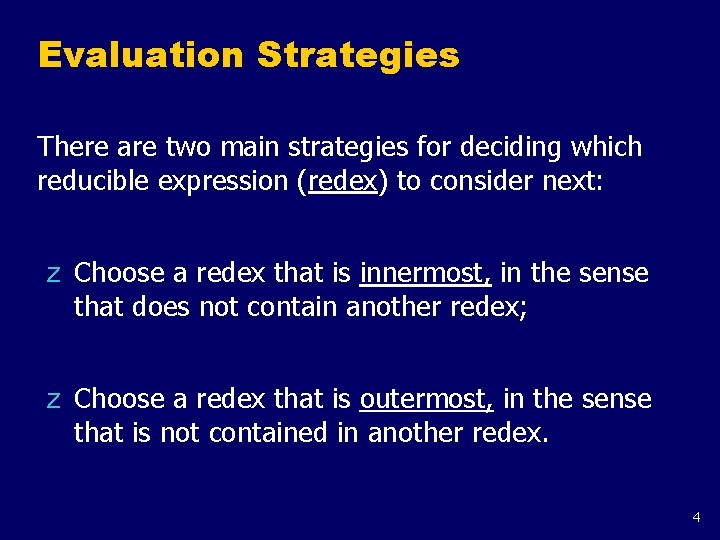
Evaluation Strategies There are two main strategies for deciding which reducible expression (redex) to consider next: z Choose a redex that is innermost, in the sense that does not contain another redex; z Choose a redex that is outermost, in the sense that is not contained in another redex. 4

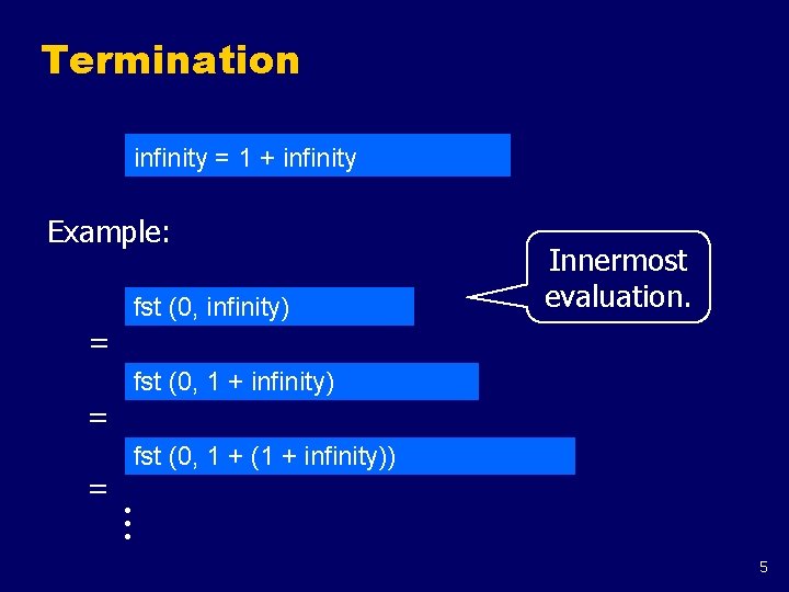
Termination infinity = 1 + infinity Example: fst (0, infinity) Innermost evaluation. = fst (0, 1 + infinity) = = fst (0, 1 + (1 + infinity)) 5

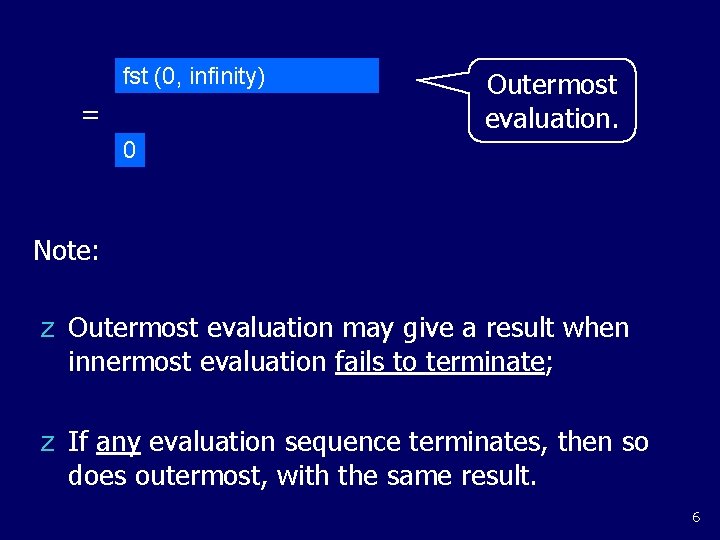
fst (0, infinity) = Outermost evaluation. 0 Note: z Outermost evaluation may give a result when innermost evaluation fails to terminate; z If any evaluation sequence terminates, then so does outermost, with the same result. 6

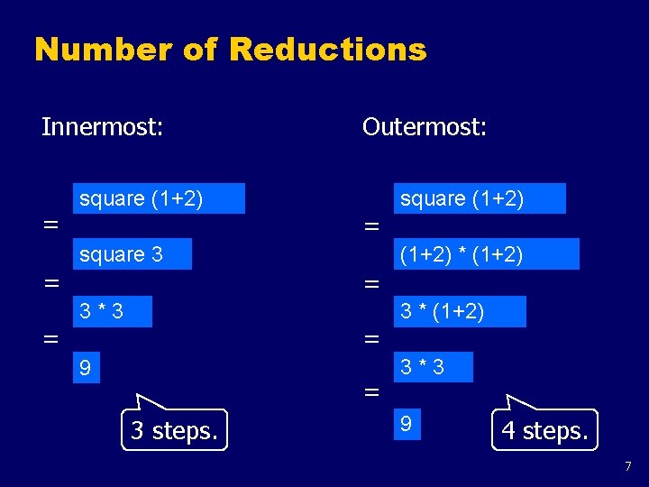
Number of Reductions Innermost: = square (1+2) Outermost: = square 3 = = square (1+2) * (1+2) = 3*3 = 9 = 3 steps. 3 * (1+2) 3*3 9 4 steps. 7

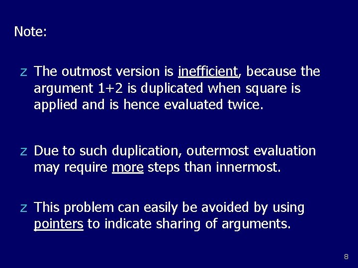
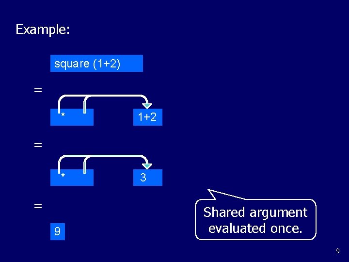
Note: z The outmost version is inefficient, because the argument 1+2 is duplicated when square is applied and is hence evaluated twice. z Due to such duplication, outermost evaluation may require more steps than innermost. z This problem can easily be avoided by using pointers to indicate sharing of arguments. 8

Example: square (1+2) = * 1+2 * 3 = = 9 Shared argument evaluated once. 9

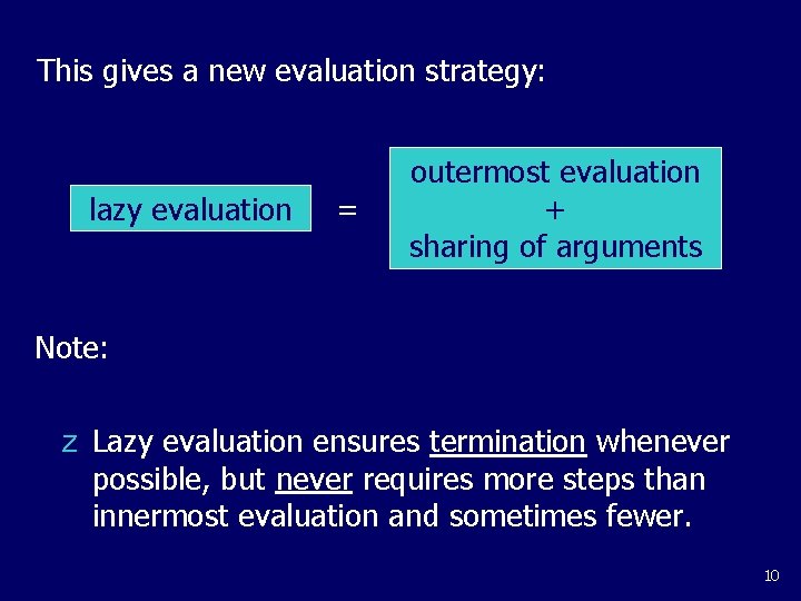
This gives a new evaluation strategy: lazy evaluation = outermost evaluation + sharing of arguments Note: z Lazy evaluation ensures termination whenever possible, but never requires more steps than innermost evaluation and sometimes fewer. 10

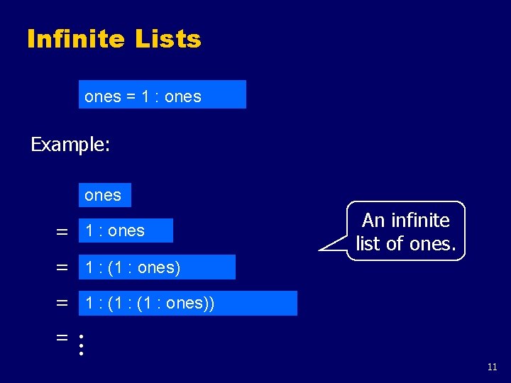
Infinite Lists ones = 1 : ones Example: ones = 1 : (1 : ones) An infinite list of ones. = 1 : (1 : ones)) = 11

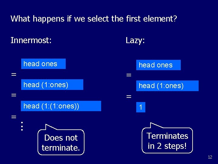
What happens if we select the first element? Innermost: Lazy: head ones = head (1: ones) = = head (1: ones)) = head (1: ones) Does not terminate. 1 Terminates in 2 steps! 12

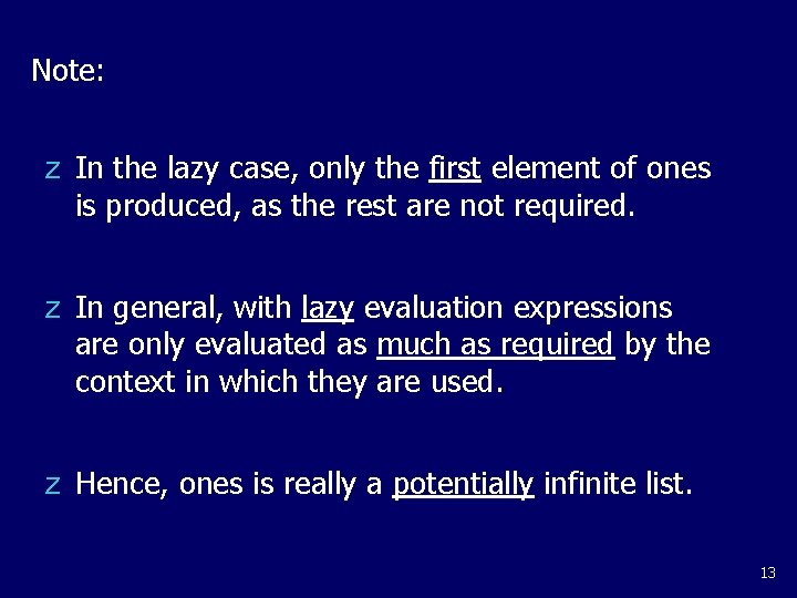
Note: z In the lazy case, only the first element of ones is produced, as the rest are not required. z In general, with lazy evaluation expressions are only evaluated as much as required by the context in which they are used. z Hence, ones is really a potentially infinite list. 13

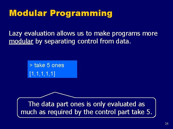
Modular Programming Lazy evaluation allows us to make programs more modular by separating control from data. > take 5 ones [1, 1, 1] The data part ones is only evaluated as much as required by the control part take 5. 14

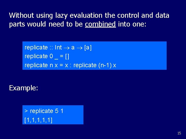
Without using lazy evaluation the control and data parts would need to be combined into one: replicate : : Int a [a] replicate 0 _ = [] replicate n x = x : replicate (n-1) x Example: > replicate 5 1 [1, 1, 1] 15

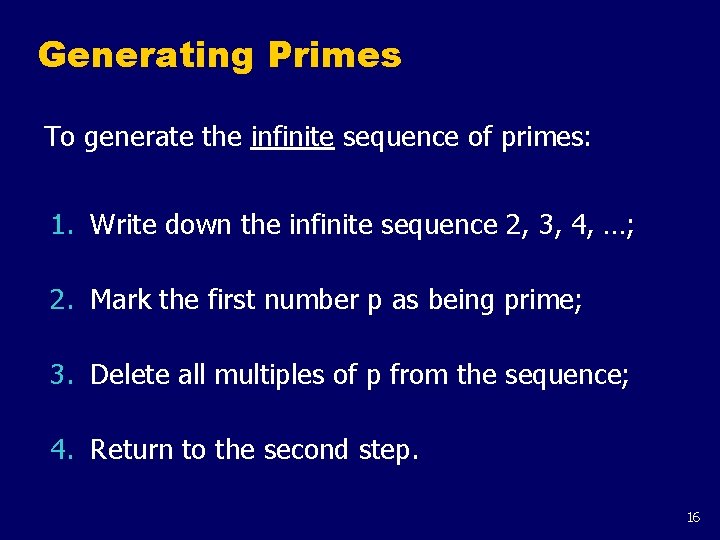
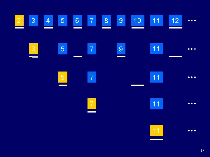
Generating Primes To generate the infinite sequence of primes: 1. Write down the infinite sequence 2, 3, 4, …; 2. Mark the first number p as being prime; 3. Delete all multiples of p from the sequence; 4. Return to the second step. 16

2 3 3 4 5 6 7 8 9 10 11 12 11 7 11 5 7 5 9 17

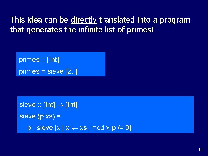
This idea can be directly translated into a program that generates the infinite list of primes! primes : : [Int] primes = sieve [2. . ] sieve : : [Int] sieve (p: xs) = p : sieve [x | x xs, mod x p /= 0] 18

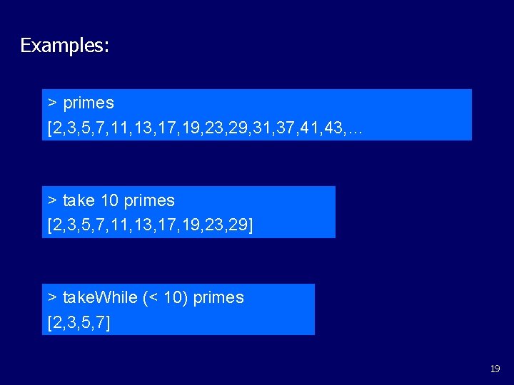
Examples: > primes [2, 3, 5, 7, 11, 13, 17, 19, 23, 29, 31, 37, 41, 43, … > take 10 primes [2, 3, 5, 7, 11, 13, 17, 19, 23, 29] > take. While (< 10) primes [2, 3, 5, 7] 19

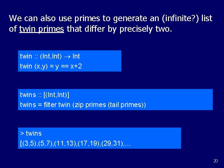
We can also use primes to generate an (infinite? ) list of twin primes that differ by precisely two. twin : : (Int, Int) Int twin (x, y) = y == x+2 twins : : [(Int, Int)] twins = filter twin (zip primes (tail primes)) > twins [(3, 5), (5, 7), (11, 13), (17, 19), (29, 31), … 20

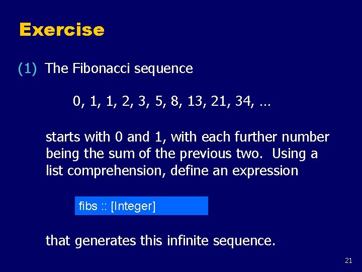
Exercise (1) The Fibonacci sequence 0, 1, 1, 2, 3, 5, 8, 13, 21, 34, … starts with 0 and 1, with each further number being the sum of the previous two. Using a list comprehension, define an expression fibs : : [Integer] that generates this infinite sequence. 21

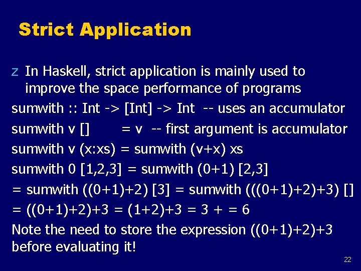
Strict Application z In Haskell, strict application is mainly used to improve the space performance of programs sumwith : : Int -> [Int] -> Int -- uses an accumulator sumwith v [] = v -- first argument is accumulator sumwith v (x: xs) = sumwith (v+x) xs sumwith 0 [1, 2, 3] = sumwith (0+1) [2, 3] = sumwith ((0+1)+2) [3] = sumwith (((0+1)+2)+3) [] = ((0+1)+2)+3 = (1+2)+3 = 3 + = 6 Note the need to store the expression ((0+1)+2)+3 before evaluating it! 22

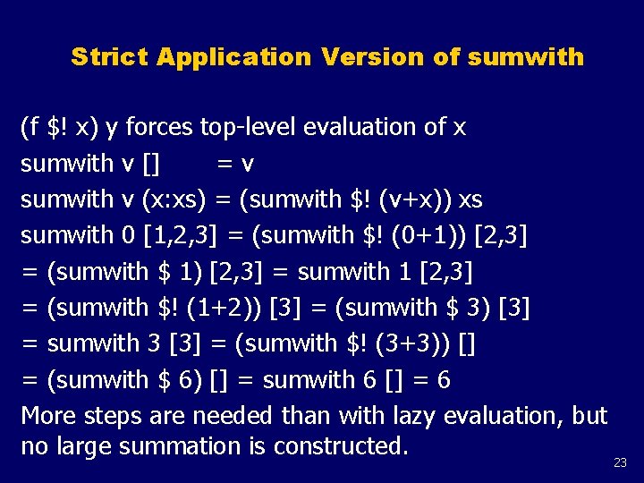
Strict Application Version of sumwith (f $! x) y forces top-level evaluation of x sumwith v [] =v sumwith v (x: xs) = (sumwith $! (v+x)) xs sumwith 0 [1, 2, 3] = (sumwith $! (0+1)) [2, 3] = (sumwith $ 1) [2, 3] = sumwith 1 [2, 3] = (sumwith $! (1+2)) [3] = (sumwith $ 3) [3] = sumwith 3 [3] = (sumwith $! (3+3)) [] = (sumwith $ 6) [] = sumwith 6 [] = 6 More steps are needed than with lazy evaluation, but no large summation is constructed. 23

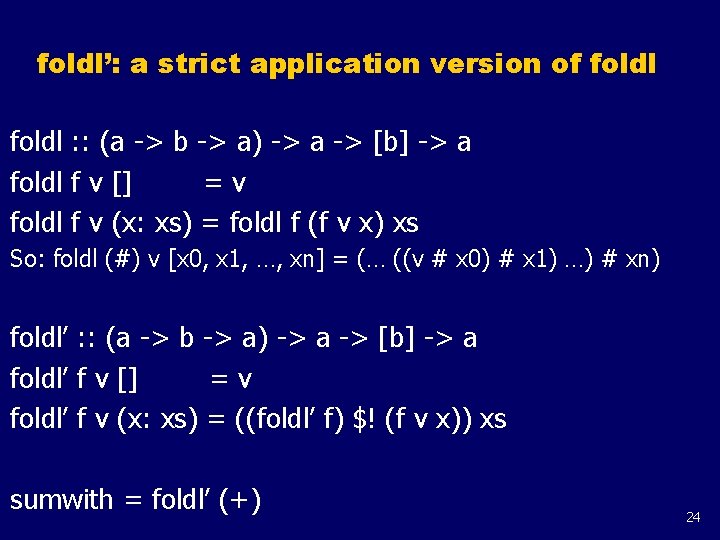
foldl’: a strict application version of foldl : : (a -> b -> a) -> a -> [b] -> a foldl f v [] =v foldl f v (x: xs) = foldl f (f v x) xs So: foldl (#) v [x 0, x 1, …, xn] = (… ((v # x 0) # x 1) …) # xn) foldl’ : : (a -> b -> a) -> a -> [b] -> a foldl’ f v [] =v foldl’ f v (x: xs) = ((foldl’ f) $! (f v x)) xs sumwith = foldl’ (+) 24