Programming for Engineers in Python Recitation 10 Plan

Programming for Engineers in Python Recitation 10

Plan �Image Processing: �Segmentation using Otsu threshold selection method �Morphological operators �Erosion �Dilation �Denoising 2

Image Processing in Python • • • 3 How to handle an image? The Python Imaging Library http: //www. pythonware. com/products/pil/ Example tutorial: http: //www. geeks 3 d. com/20100930/tutorial-firststeps-with-pil-python-imaging-library The Image Module: http: //www. pythonware. com/library/pil/handbook/image. htm Capacities: • Read / write images • Display image • Basic image processing

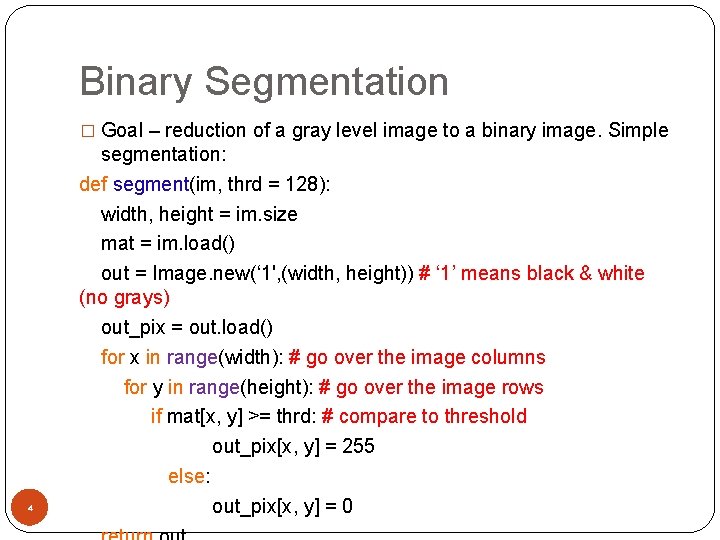
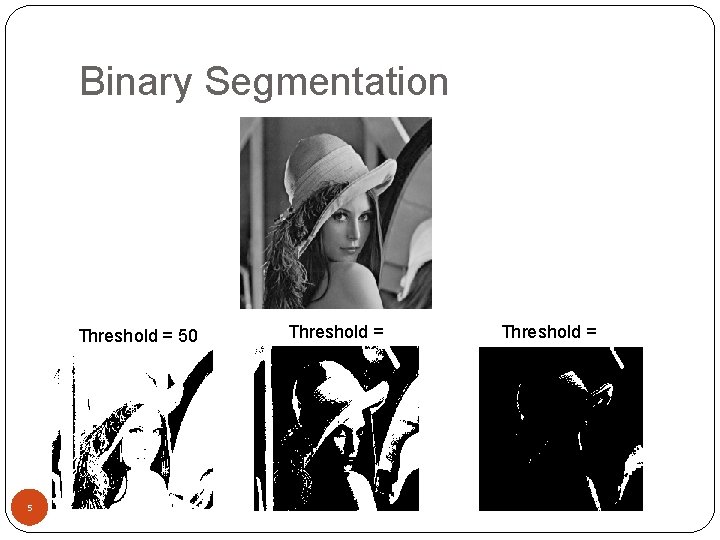
Binary Segmentation � Goal – reduction of a gray level image to a binary image. Simple 4 segmentation: def segment(im, thrd = 128): width, height = im. size mat = im. load() out = Image. new(‘ 1', (width, height)) # ‘ 1’ means black & white (no grays) out_pix = out. load() for x in range(width): # go over the image columns for y in range(height): # go over the image rows if mat[x, y] >= thrd: # compare to threshold out_pix[x, y] = 255 else: out_pix[x, y] = 0

Binary Segmentation Threshold = 50 5 Threshold = 128 Threshold = 200

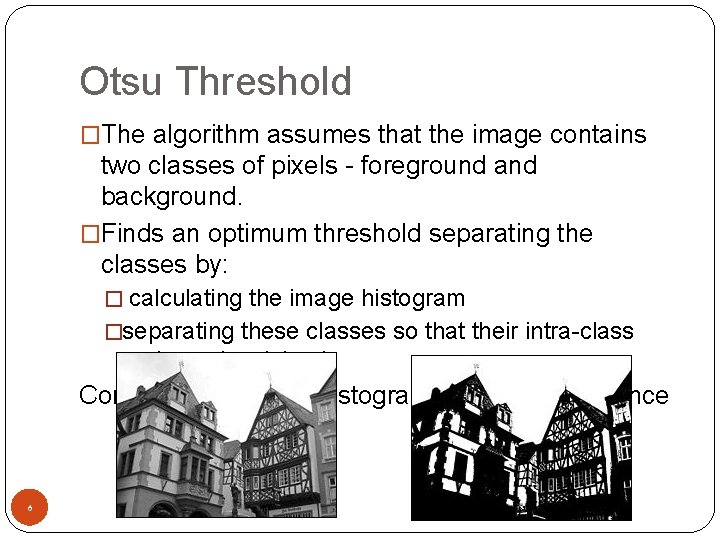
Otsu Threshold �The algorithm assumes that the image contains two classes of pixels - foreground and background. �Finds an optimum threshold separating the classes by: � calculating the image histogram �separating these classes so that their intra-class variance is minimal. Coming next: image histogram, intra-class variance 6

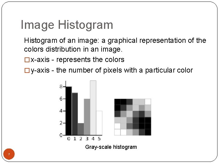
Image Histogram of an image: a graphical representation of the colors distribution in an image. � x-axis - represents the colors � y-axis - the number of pixels with a particular color Gray-scale histogram 7

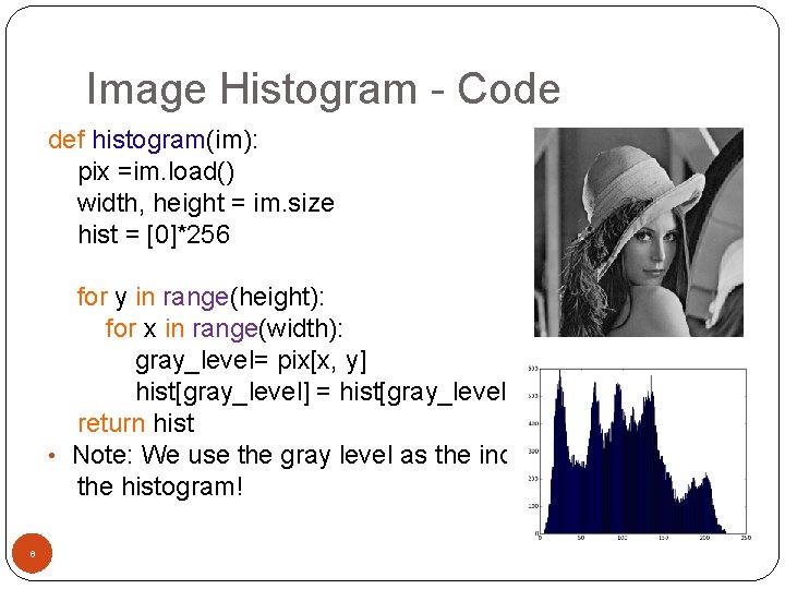
Image Histogram - Code def histogram(im): pix =im. load() width, height = im. size hist = [0]*256 for y in range(height): for x in range(width): gray_level= pix[x, y] hist[gray_level] = hist[gray_level]+1 return hist • Note: We use the gray level as the index of the histogram! 8

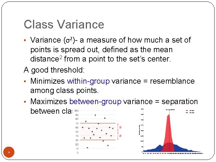
Class Variance • Variance (σ2)- a measure of how much a set of points is spread out, defined as the mean distance 2 from a point to the set’s center. A good threshold: • Minimizes within-group variance = resemblance among class points. • Maximizes between-group variance = separation between class centers. 9

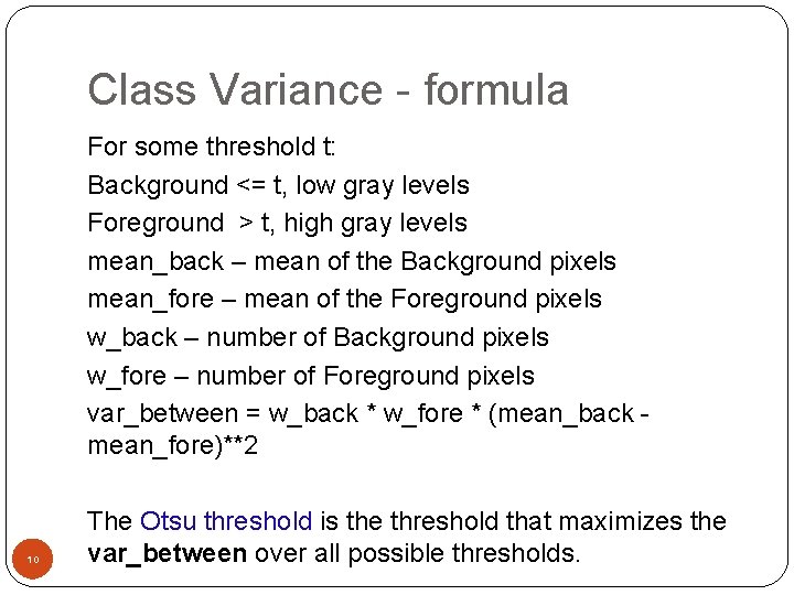
Class Variance - formula For some threshold t: Background <= t, low gray levels Foreground > t, high gray levels mean_back – mean of the Background pixels mean_fore – mean of the Foreground pixels w_back – number of Background pixels w_fore – number of Foreground pixels var_between = w_back * w_fore * (mean_back mean_fore)**2 10 The Otsu threshold is the threshold that maximizes the var_between over all possible thresholds.

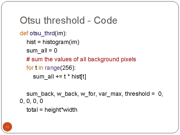
Otsu threshold - Code def otsu_thrd(im): hist = histogram(im) sum_all = 0 # sum the values of all background pixels for t in range(256): sum_all += t * hist[t] sum_back, w_for, var_max, threshold = 0, 0, 0 total = height*width 11

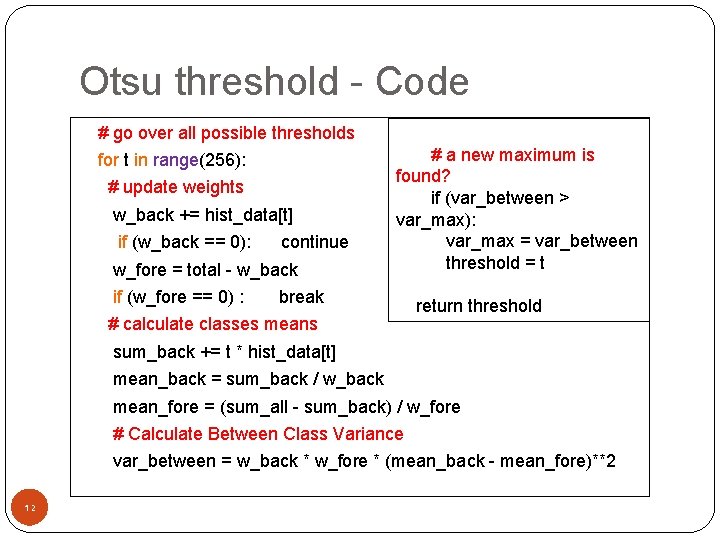
Otsu threshold - Code # go over all possible thresholds for t in range(256): # update weights w_back += hist_data[t] if (w_back == 0): continue w_fore = total - w_back if (w_fore == 0) : # a new maximum is found? if (var_between > var_max): var_max = var_between threshold = t break # calculate classes means return threshold sum_back += t * hist_data[t] mean_back = sum_back / w_back mean_fore = (sum_all - sum_back) / w_fore # Calculate Between Class Variance var_between = w_back * w_fore * (mean_back - mean_fore)**2 12

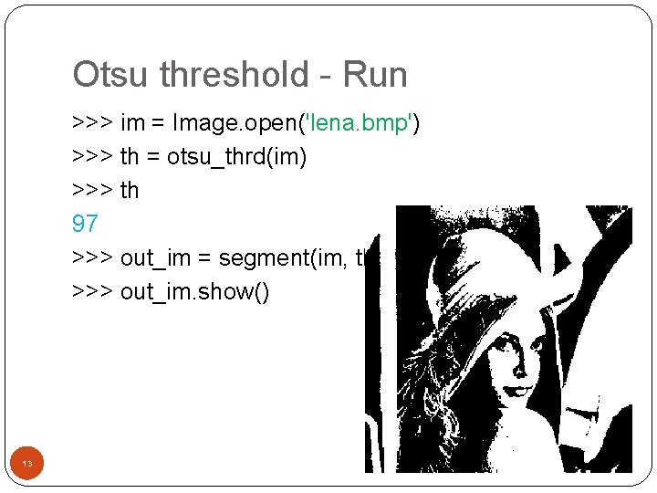
Otsu threshold - Run >>> im = Image. open('lena. bmp') >>> th = otsu_thrd(im) >>> th 97 >>> out_im = segment(im, th) >>> out_im. show() 13

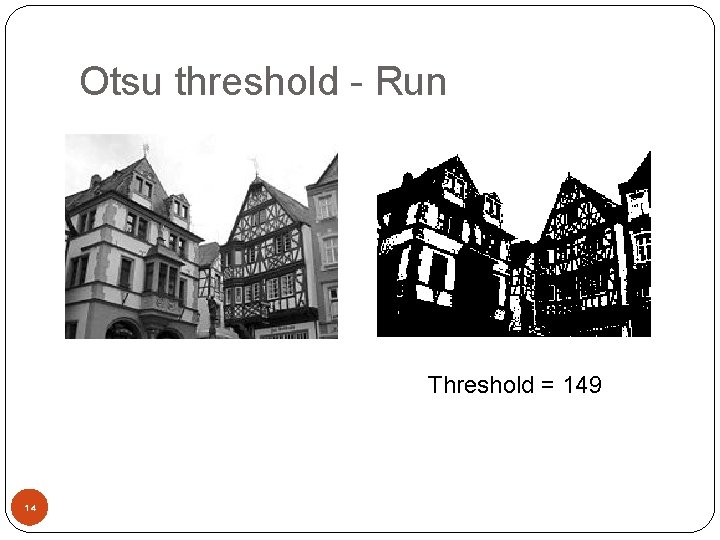
Otsu threshold - Run Threshold = 149 14

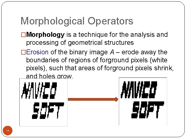
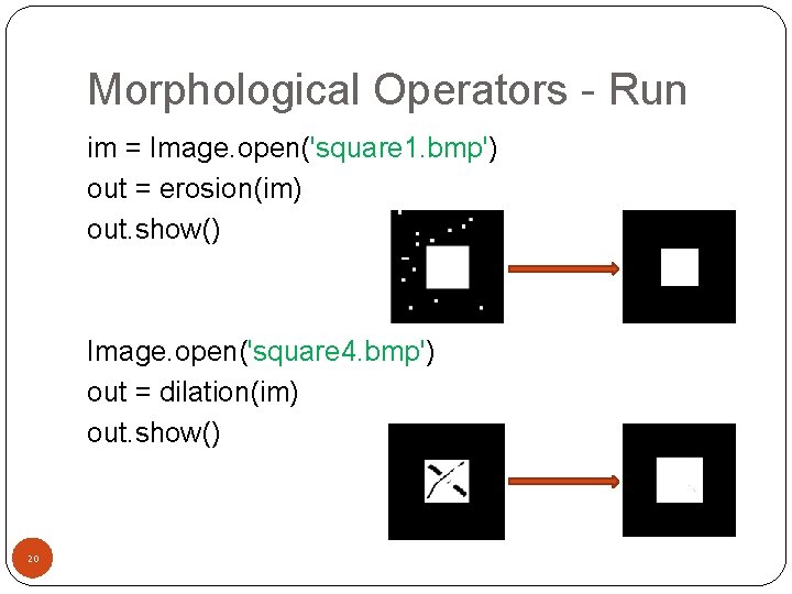
Morphological Operators �Morphology is a technique for the analysis and processing of geometrical structures �Erosion of the binary image A – erode away the boundaries of regions of forground pixels (white pixels), such that areas of forground pixels shrink, and holes grow. 15

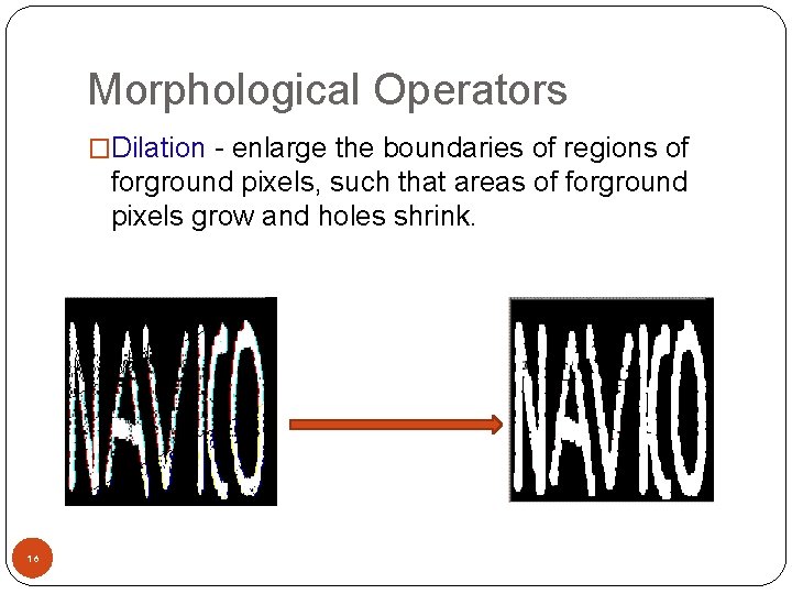
Morphological Operators �Dilation - enlarge the boundaries of regions of forground pixels, such that areas of forground pixels grow and holes shrink. 16

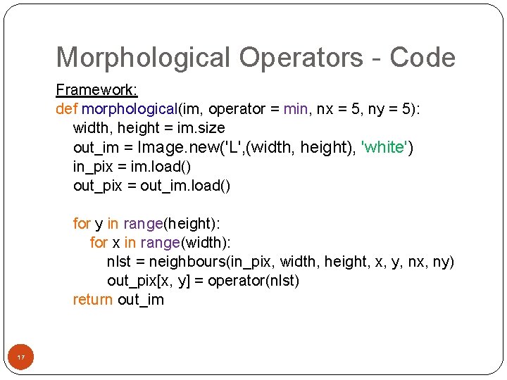
Morphological Operators - Code Framework: def morphological(im, operator = min, nx = 5, ny = 5): width, height = im. size out_im = Image. new('L', (width, height), 'white') in_pix = im. load() out_pix = out_im. load() for y in range(height): for x in range(width): nlst = neighbours(in_pix, width, height, x, y, nx, ny) out_pix[x, y] = operator(nlst) return out_im 17

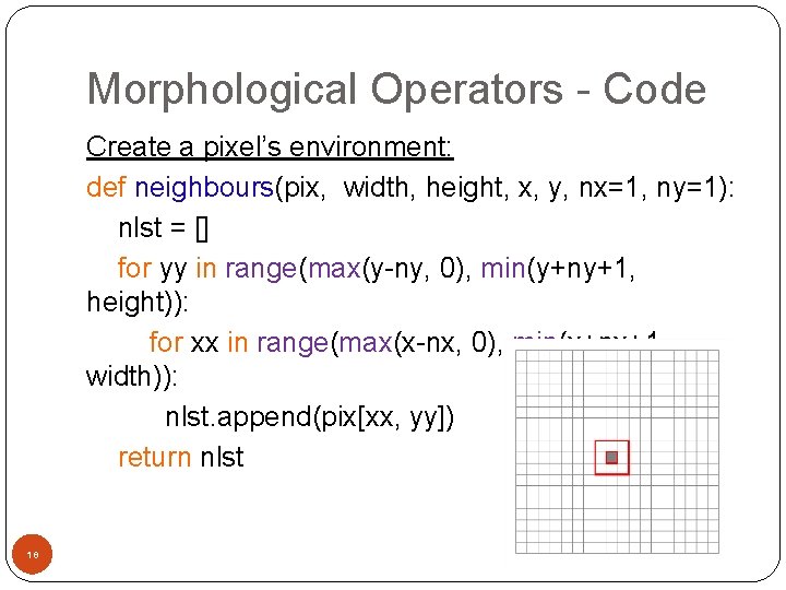
Morphological Operators - Code Create a pixel’s environment: def neighbours(pix, width, height, x, y, nx=1, ny=1): nlst = [] for yy in range(max(y-ny, 0), min(y+ny+1, height)): for xx in range(max(x-nx, 0), min(x+nx+1, width)): nlst. append(pix[xx, yy]) return nlst 18

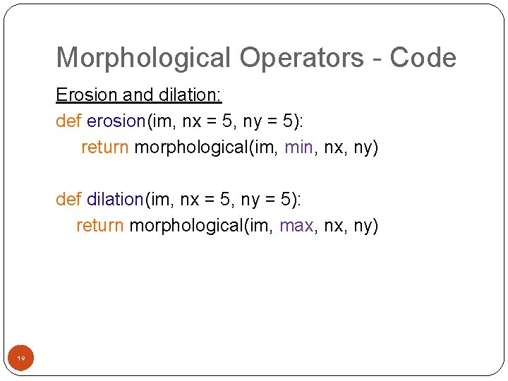
Morphological Operators - Code Erosion and dilation: def erosion(im, nx = 5, ny = 5): return morphological(im, min, nx, ny) def dilation(im, nx = 5, ny = 5): return morphological(im, max, ny) 19

Morphological Operators - Run im = Image. open('square 1. bmp') out = erosion(im) out. show() Image. open('square 4. bmp') out = dilation(im) out. show() 20

Dilation for Edge Detection # find the differences between two images def diff(im 1, im 2): out = Image. new('L', im 1. size, 'white') out_pix = out. load() p 1 = im 1. load() p 2 = im 2. load() width, height = im 1. size for x in range(width): for y in range(height): out_pix[x, y] = abs(p 1[x, y] - p 2[x, y]) return out 21

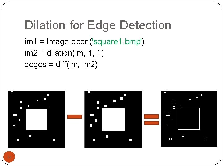
Dilation for Edge Detection im 1 = Image. open('square 1. bmp') im 2 = dilation(im, 1, 1) edges = diff(im, im 2) 22

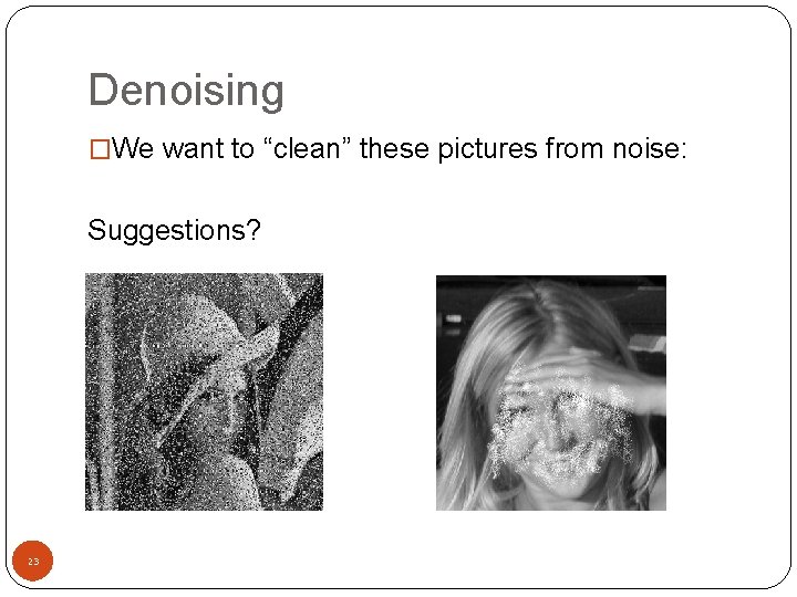
Denoising �We want to “clean” these pictures from noise: Suggestions? 23

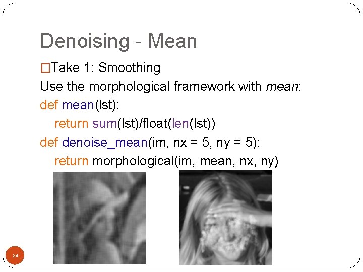
Denoising - Mean �Take 1: Smoothing Use the morphological framework with mean: def mean(lst): return sum(lst)/float(len(lst)) def denoise_mean(im, nx = 5, ny = 5): return morphological(im, mean, nx, ny) 24

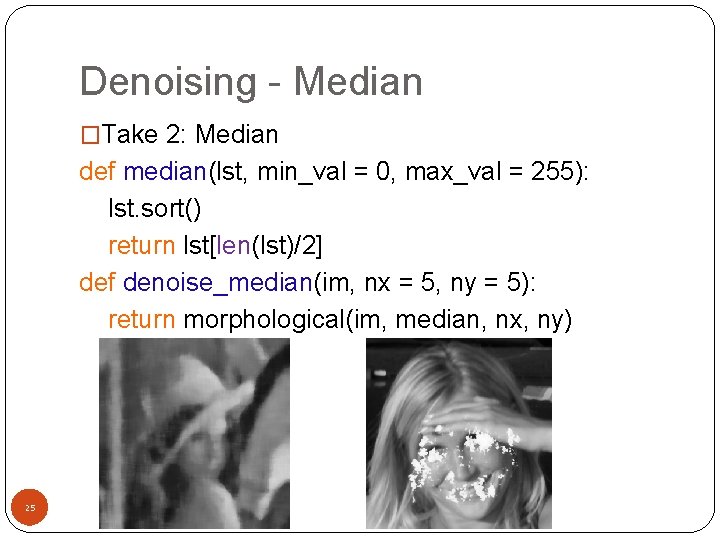
Denoising - Median �Take 2: Median def median(lst, min_val = 0, max_val = 255): lst. sort() return lst[len(lst)/2] def denoise_median(im, nx = 5, ny = 5): return morphological(im, median, nx, ny) 25

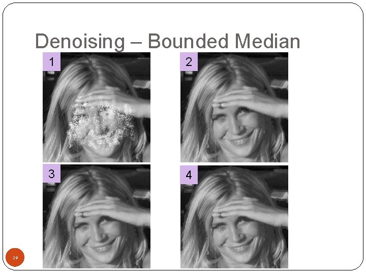
Denoising - Median �Can we do better? �Idea – the ‘salt’ is (almost) white, the ‘pepper’ is (almost) black. We can change very bright or very dark pixels only! To calculate the median, we will use only neighboring pixels that are not close to the pixel we change. àThe noisy pixels surrounded by ‘normal’ pixels will be fixed. àContinue iteratively 26

Denoising – Bounded Median def median(lst, min_val = 0, max_val = 255): lst. sort() new_lst = [i for i in lst if (i >= min_val and i <= max_val)] if new_lst: return new_lst[len(new_lst)/2] else: return lst[len(lst)/2] 27 def fix_white(lst, k = 200): center = len(lst)/2 if lst[center] > k: return median(lst, max_val = k) else: return lst[center] def fix_black(lst, b = 50): center = len(lst)/2 if lst[center] < b: return median(lst, min_val = b) else: return lst[center]

Denoising – Bounded Median def denoise_bounded_median(im, nx = 3, ny = 3): for i in range(3): im = morphological(im, fix_white, nx, ny) im = morphological(im, fix_black, nx, ny) return im 28

Denoising – Bounded Median 29 1 2 3 4