Programming Biology Andrew Phillips with Luca Cardelli Microsoft

Programming Biology Andrew Phillips with Luca Cardelli Microsoft Research, Cambridge UK

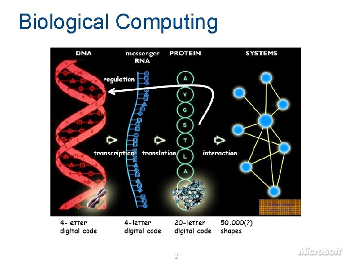
Biological Computing 2

Modelling Biology The Human Genome project: Map out the complete genetic code in humans To understand predict gene and protein behaviour Like reading the source code of a computer program. . . But functional meaning of the code is still a mystery! Systems Biology: Understand precisely describe the behaviour of biological systems Two complementary approaches: Look at experimental results and infer general system properties Build detailed models of systems and test these in the lab Biological Modelling: Conduct virtual experiments, saving time and money. Need tools for modelling complex parallel systems. Should also scale up to very large systems. The beginnings of a biological programming language. . . 3

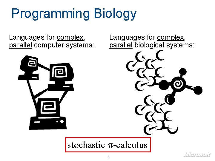
Programming Biology Languages for complex, parallel computer systems: Languages for complex, parallel biological systems: stochastic p-calculus 4

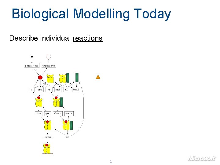
Biological Modelling Today Describe individual reactions 5

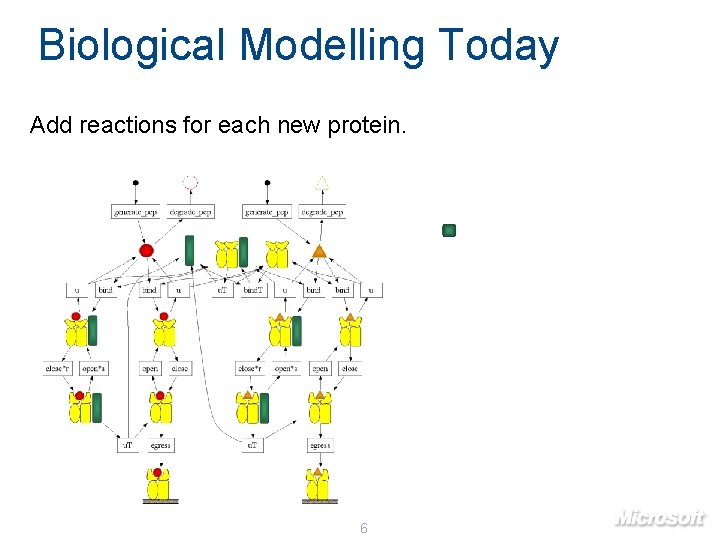
Biological Modelling Today Add reactions for each new protein. 6

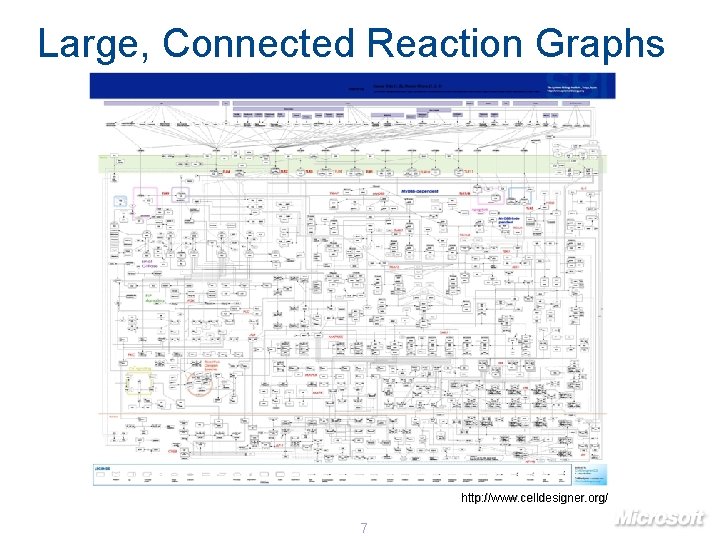
Large, Connected Reaction Graphs http: //www. celldesigner. org/ 7

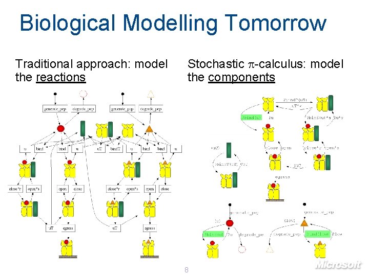
Biological Modelling Tomorrow Traditional approach: model the reactions Stochastic p-calculus: model the components 8

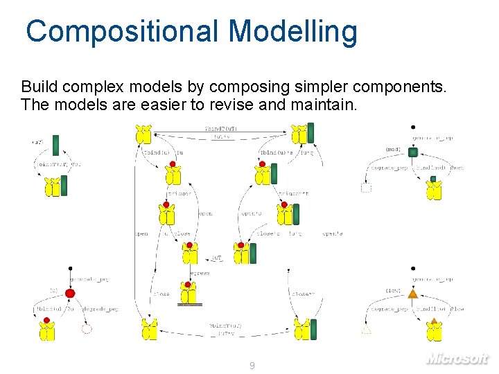
Compositional Modelling Build complex models by composing simpler components. The models are easier to revise and maintain. 9

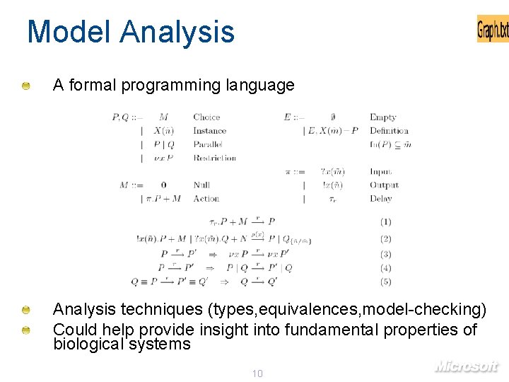
Model Analysis A formal programming language Analysis techniques (types, equivalences, model-checking) Could help provide insight into fundamental properties of biological systems 10

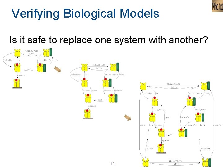
Verifying Biological Models Is it safe to replace one system with another? 11

Outline Programming Language Development Introduction to Stochastic Pi-calculus Programming Gene Networks Programming an Immune System Pathway 12

Programming Language Development Initial Challenges

Related Work Stochastic p-calculus proposed by [Priami, 1995] Used to simulate a range of biological systems: RTK MAPK pathway [Regev et al. , 2001] Gene Regulation by positive Feedback [Priami et al. , 2001] Cell Cycle Control in Eukaryotes [Lecca and Priami, 2003] First simulator for stochastic p-calculus [Bio. SPI] A subset of p-calculus with limited choice Compiles a calculus process to an FCP procedure Executed by the FCP Logix platform [Silverman et al. , 1987] 14

Graphical Stochastic p-calculus Display stochastic p-calculus models as graphs [Phillips and Cardelli, 2005] Helps make the stochastic p-calculus more accessible Defined a graphical calculus and graphical execution model Proved equivalent to the stochastic p-calculus [Phillips, Cardelli and Castagna, 2006] let g. Low() = delay@g_pep; (Low() | g. Low()) and Low()= ( new low@u. Low: chan do !pep(low); ? low; Low() or delay@d_pep ) let g. Med() = delay@g_pep; (Med() | g. Med()) and Med()= ( new med@u. Med: chan do !pep(med); ? med; Med() or delay@d_pep ) let g. High() = delay@g_pep; (High() | g. High()) and High()= ( new high@u. High: chan do !pep(high); ? high; High() or delay@d_pep ) let g. MHC() = delay@g_MHC; (g. MHC() | MHCo() ) and g. TPN() = delay@g_TPN; ( g. TPN() | TPN() ) and TPN()= ( new u. T@unbind_TPN: chan do !tpn(u. T); ? u. T; TPN() or delay@degrade_TPN ) and MHCo()= do ? pep(u); MHCc_pep(u) or ? tpn(u. T); MHCo_TPN(u. T) or delay@degrade_MHCo and MHCc_pep(u: chan) = do delay@egress; MHCe_pep(u) or !u; MHCo() and MHCe_pep(u: chan) = delay@degrade_MHCe PROVED EQUIVALENT and MHCo_TPN(u. T: chan)= do ? pep(u)*a; MHCc_TPN_pep(u, u. T) or !u. T*v; MHCo() and MHCc_TPN_pep(u: chan, u. T: chan)= do !u. T; MHCc_pep(u) or !u*q; MHCo_TPN(u. T) 15

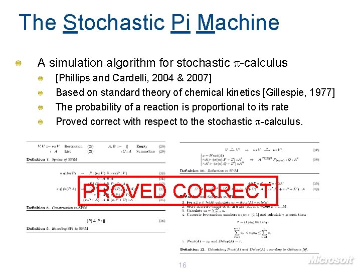
The Stochastic Pi Machine A simulation algorithm for stochastic p-calculus [Phillips and Cardelli, 2004 & 2007] Based on standard theory of chemical kinetics [Gillespie, 1977] The probability of a reaction is proportional to its rate Proved correct with respect to the stochastic p-calculus. PROVED CORRECT 16

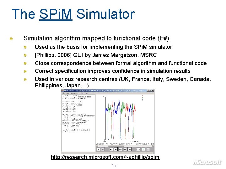
The SPi. M Simulator Simulation algorithm mapped to functional code (F#) Used as the basis for implementing the SPi. M simulator. [Phillips, 2006] GUI by James Margetson, MSRC Close correspondence between formal algorithm and functional code Correct specification improves confidence in simulation results Used in various research centres (UK, France, Italy, Sweden, Canada, Philippines, Japan, . . . ) http: //research. microsoft. com/~aphillip/spim 17

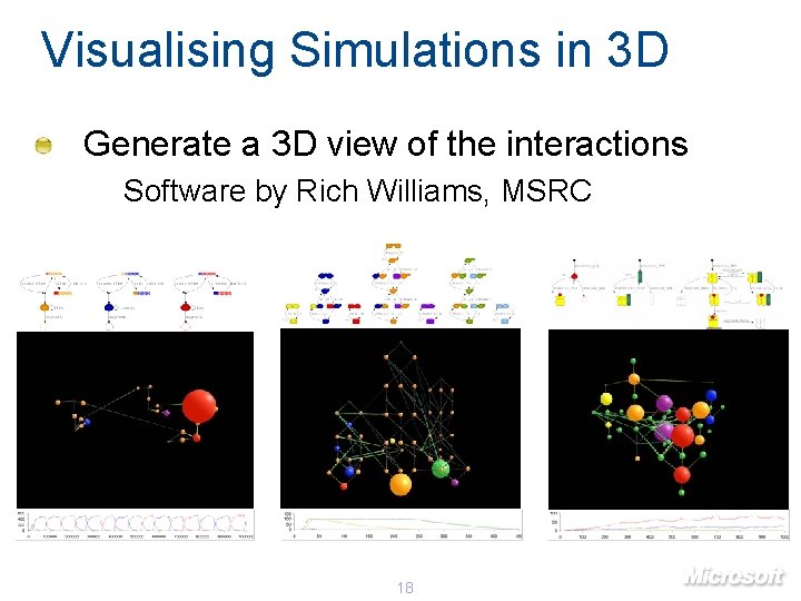
Visualising Simulations in 3 D Generate a 3 D view of the interactions Software by Rich Williams, MSRC 18

Introduction to Stochastic Pi-calculus Chemical Reactions

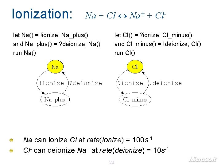
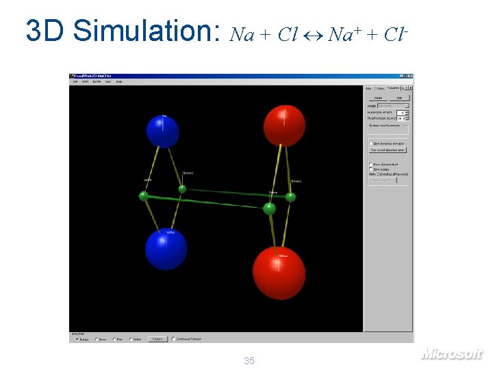
Ionization: Na + Cl Na+ + Cl- let Na() = !ionize; Na_plus() and Na_plus() = ? deionize; Na() run Na() let Cl() = ? ionize; Cl_minus() and Cl_minus() = !deionize; Cl() run Cl() Na can ionize Cl at rate(ionize) = 100 s-1 Cl- can deionize Na+ at rate(deionize) = 10 s-1 20

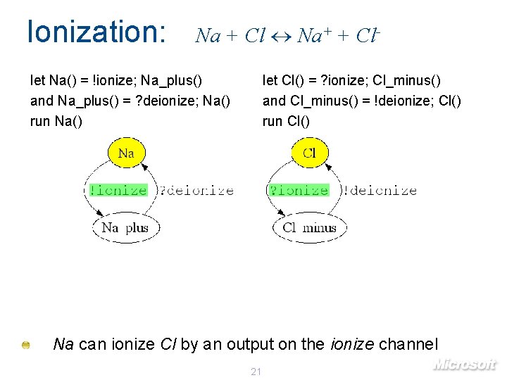
Ionization: Na + Cl Na+ + Cl- let Na() = !ionize; Na_plus() and Na_plus() = ? deionize; Na() run Na() let Cl() = ? ionize; Cl_minus() and Cl_minus() = !deionize; Cl() run Cl() Na can ionize Cl by an output on the ionize channel 21

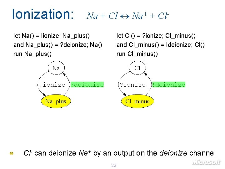
Ionization: Na + Cl Na+ + Cl- let Na() = !ionize; Na_plus() and Na_plus() = ? deionize; Na() run Na_plus() let Cl() = ? ionize; Cl_minus() and Cl_minus() = !deionize; Cl() run Cl_minus() Cl- can deionize Na+ by an output on the deionize channel 22

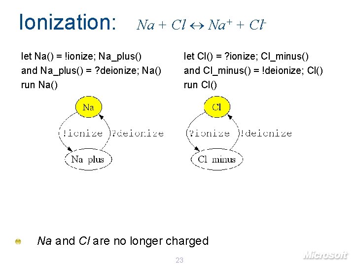
Ionization: Na + Cl Na+ + Cl- let Na() = !ionize; Na_plus() and Na_plus() = ? deionize; Na() run Na() let Cl() = ? ionize; Cl_minus() and Cl_minus() = !deionize; Cl() run Cl() Na and Cl are no longer charged 23

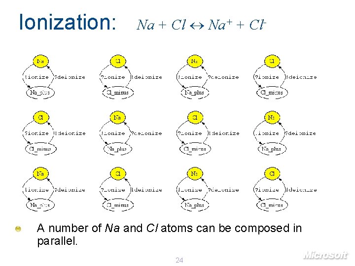
Ionization: Na + Cl Na+ + Cl- A number of Na and Cl atoms can be composed in parallel. 24

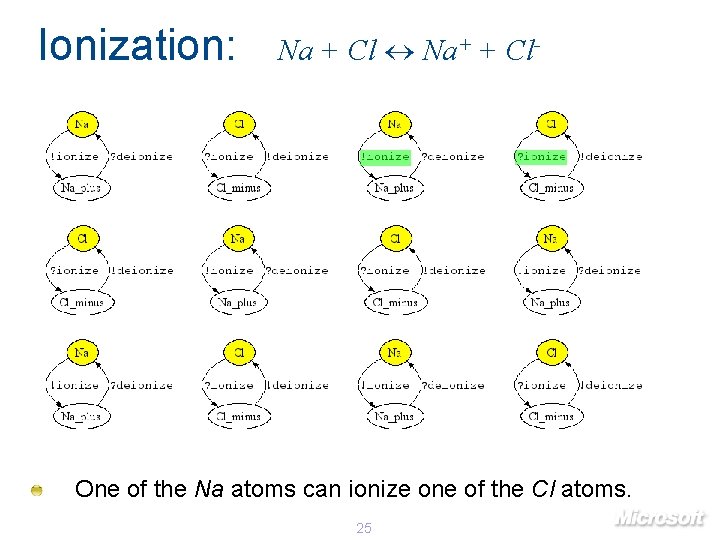
Ionization: Na + Cl Na+ + Cl- One of the Na atoms can ionize one of the Cl atoms. 25

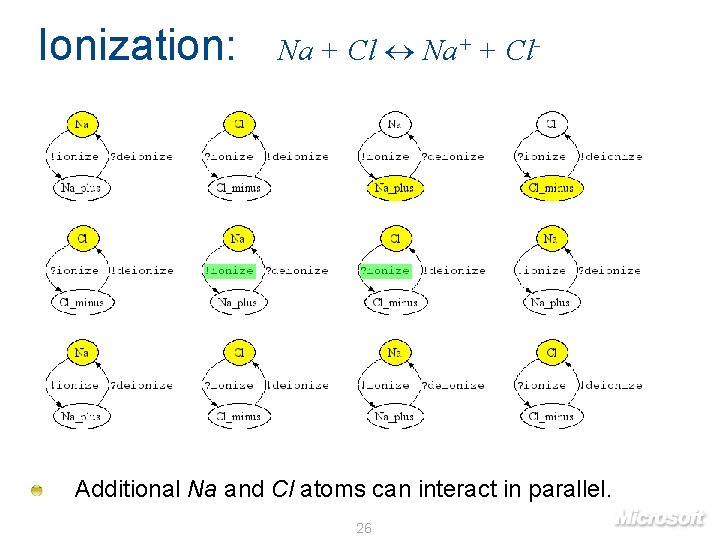
Ionization: Na + Cl Na+ + Cl- Additional Na and Cl atoms can interact in parallel. 26

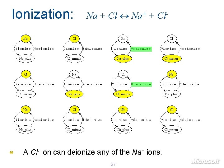
Ionization: Na + Cl Na+ + Cl- A Cl- ion can deionize any of the Na+ ions. 27

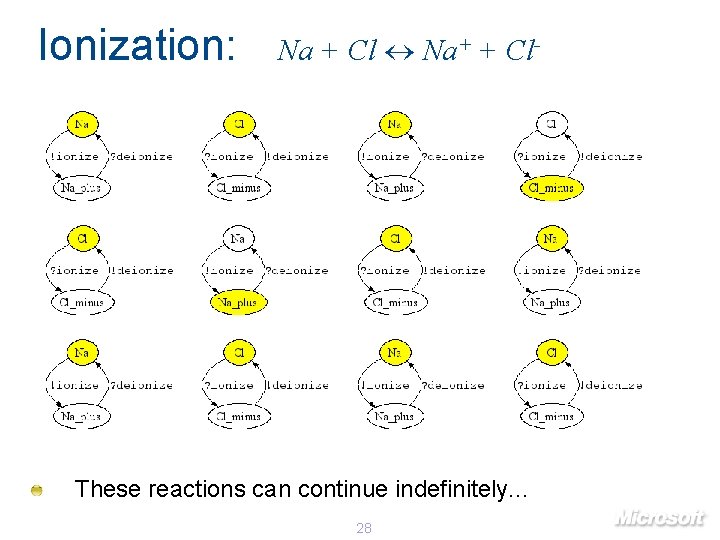
Ionization: Na + Cl Na+ + Cl- These reactions can continue indefinitely. . . 28

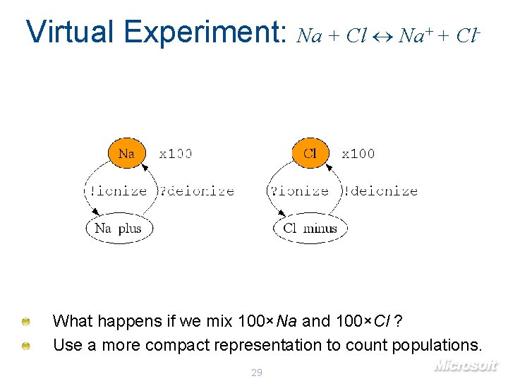
Virtual Experiment: Na + Cl Na+ + Cl- What happens if we mix 100×Na and 100×Cl ? Use a more compact representation to count populations. 29

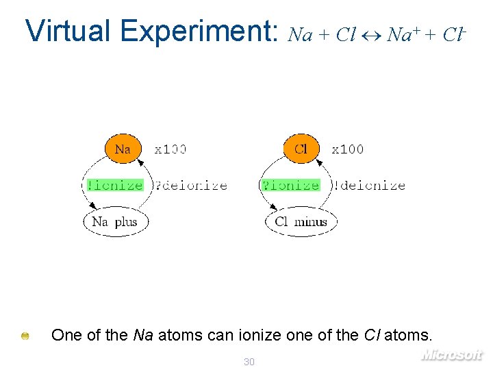
Virtual Experiment: Na + Cl Na+ + Cl- One of the Na atoms can ionize one of the Cl atoms. 30

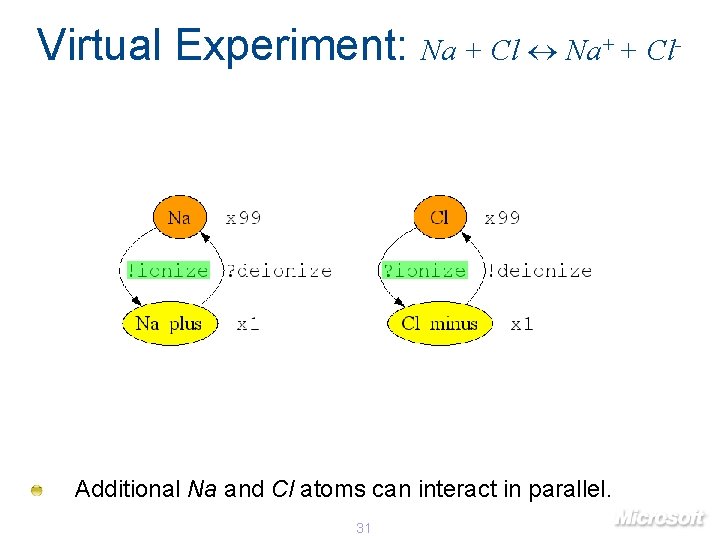
Virtual Experiment: Na + Cl Na+ + Cl- Additional Na and Cl atoms can interact in parallel. 31

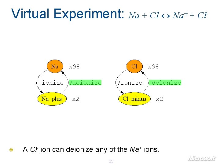
Virtual Experiment: Na + Cl Na+ + Cl- A Cl- ion can deionize any of the Na+ ions. 32

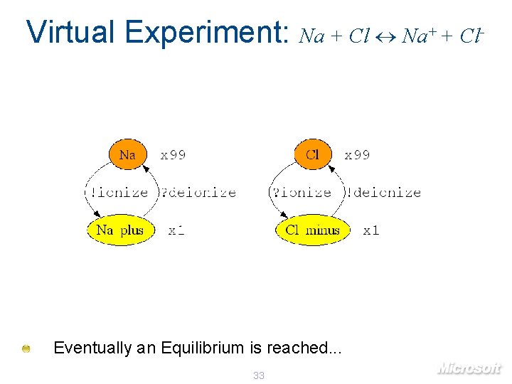
Virtual Experiment: Na + Cl Na+ + Cl- Eventually an Equilibrium is reached. . . 33

Virtual Experiment: Na + Cl Na+ + Cl- At equilibrium: 100×[Na][Cl] = 10×[Na+][Cl-] Approximately 76×Na and 24×Na+ 34

3 D Simulation: Na + Cl Na+ + Cl- 35

Gene Networks with Luca Cardelli (MSR Cambridge) Ralf Blossey (IRI Lille)

Programming a Biological Clock 37

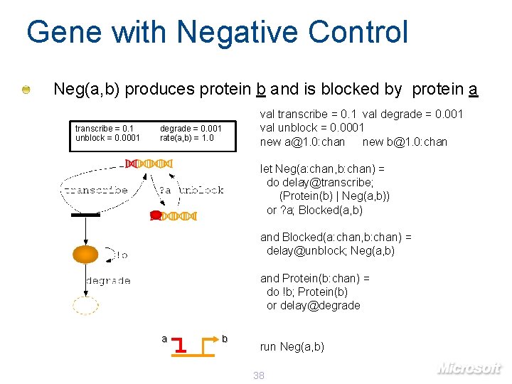
Gene with Negative Control Neg(a, b) produces protein b and is blocked by protein a transcribe = 0. 1 unblock = 0. 0001 degrade = 0. 001 rate(a, b) = 1. 0 val transcribe = 0. 1 val degrade = 0. 001 val unblock = 0. 0001 new a@1. 0: chan new b@1. 0: chan let Neg(a: chan, b: chan) = do delay@transcribe; (Protein(b) | Neg(a, b)) or ? a; Blocked(a, b) and Blocked(a: chan, b: chan) = delay@unblock; Neg(a, b) and Protein(b: chan) = do !b; Protein(b) or delay@degrade a b run Neg(a, b) 38

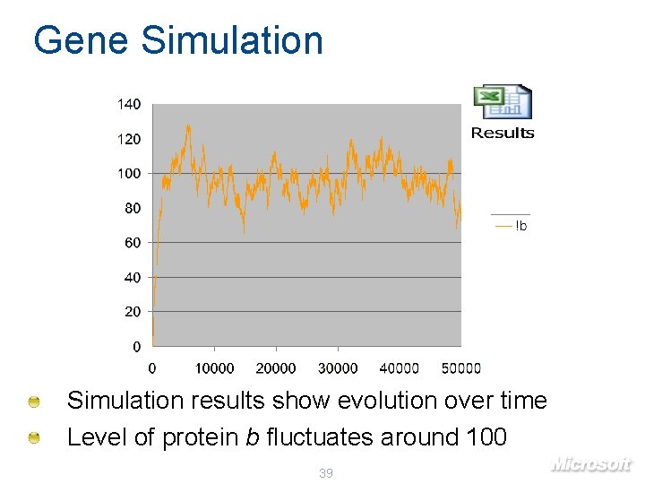
Gene Simulation results show evolution over time Level of protein b fluctuates around 100 39

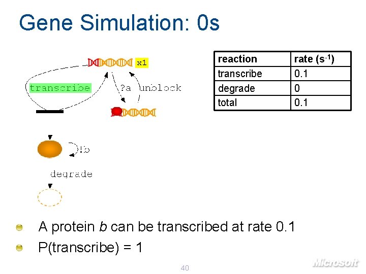
Gene Simulation: 0 s reaction transcribe degrade total x 1 rate (s-1) 0. 1 0 0. 1 A protein b can be transcribed at rate 0. 1 P(transcribe) = 1 40

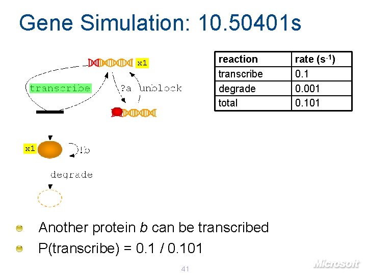
Gene Simulation: 10. 50401 s reaction transcribe degrade total x 1 Another protein b can be transcribed P(transcribe) = 0. 1 / 0. 101 41 rate (s-1) 0. 1 0. 001 0. 101

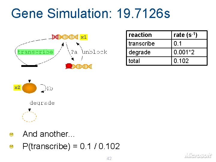
Gene Simulation: 19. 7126 s reaction transcribe degrade total x 1 x 2 And another. . . P(transcribe) = 0. 1 / 0. 102 42 rate (s-1) 0. 1 0. 001*2 0. 102

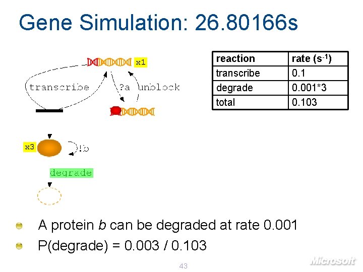
Gene Simulation: 26. 80166 s reaction transcribe degrade total x 1 rate (s-1) 0. 1 0. 001*3 0. 103 x 3 A protein b can be degraded at rate 0. 001 P(degrade) = 0. 003 / 0. 103 43

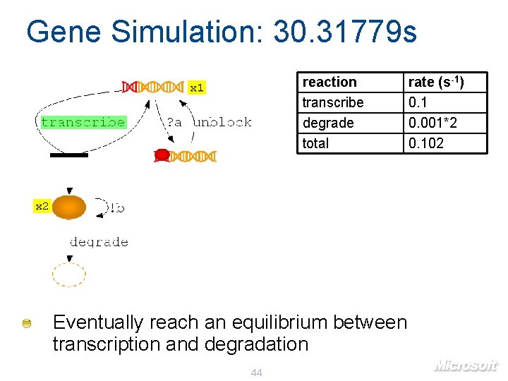
Gene Simulation: 30. 31779 s reaction transcribe degrade total x 1 x 2 Eventually reach an equilibrium between transcription and degradation 44 rate (s-1) 0. 1 0. 001*2 0. 102

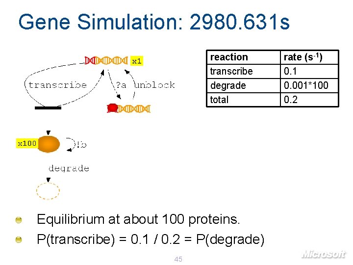
Gene Simulation: 2980. 631 s reaction transcribe degrade total x 100 Equilibrium at about 100 proteins. P(transcribe) = 0. 1 / 0. 2 = P(degrade) 45 rate (s-1) 0. 1 0. 001*100 0. 2

Repressilator [Elowitz and Leibler, 2000] A gene network engineered in live bacteria. Modelled as a simple combination of Neg gates: ( Neg(lac, tet) | Neg(tet, lambda) | Neg(lambda, lac) | Neg(tet, gfp) ) © 2000 Elowitz, M. B. , Leibler. S. A Synthetic Oscillatory Network of Transcriptional Regulators. Nature 403: 335 -338. 46

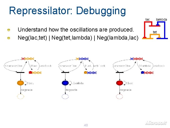
Repressilator: Debugging lac Understand how the oscillations are produced. Neg(lac, tet) | Neg(tet, lambda) | Neg(lambda, lac) 48 lambda tet

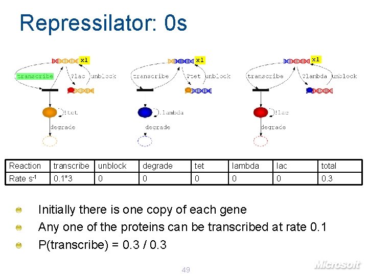
Repressilator: 0 s x 1 x 1 Reaction transcribe unblock degrade tet lambda lac total Rate s-1 0. 1*3 0 0 0. 3 Initially there is one copy of each gene Any one of the proteins can be transcribed at rate 0. 1 P(transcribe) = 0. 3 / 0. 3 49

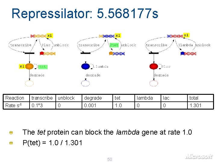
Repressilator: 5. 568177 s x 1 x 1 Reaction transcribe unblock degrade tet lambda lac total Rate s-1 0. 1*3 0 0. 001 1. 0 0 0 1. 301 The tet protein can block the lambda gene at rate 1. 0 P(tet) = 1. 0 / 1. 301 50

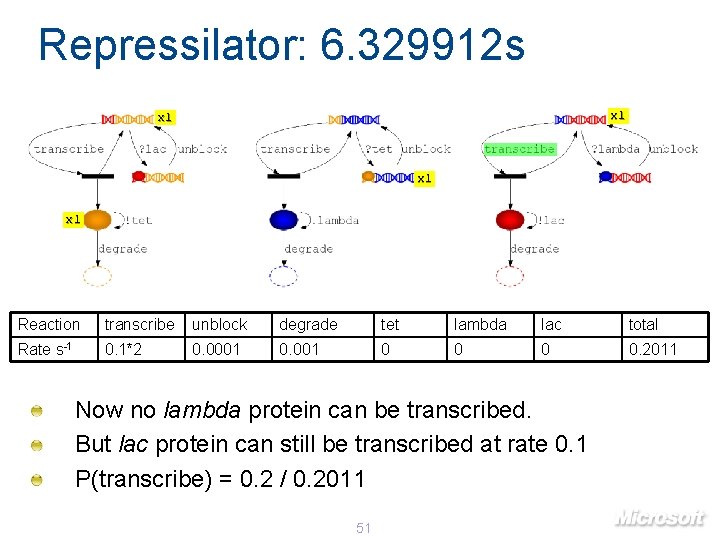
Repressilator: 6. 329912 s x 1 x 1 Reaction transcribe unblock degrade tet lambda lac total Rate s-1 0. 1*2 0. 0001 0 0. 2011 Now no lambda protein can be transcribed. But lac protein can still be transcribed at rate 0. 1 P(transcribe) = 0. 2 / 0. 2011 51

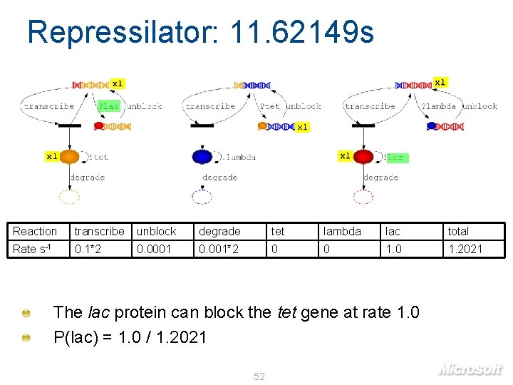
Repressilator: 11. 62149 s x 1 x 1 x 1 Reaction transcribe unblock degrade tet lambda lac total Rate s-1 0. 1*2 0. 0001 0. 001*2 0 0 1. 2021 The lac protein can block the tet gene at rate 1. 0 P(lac) = 1. 0 / 1. 2021 52

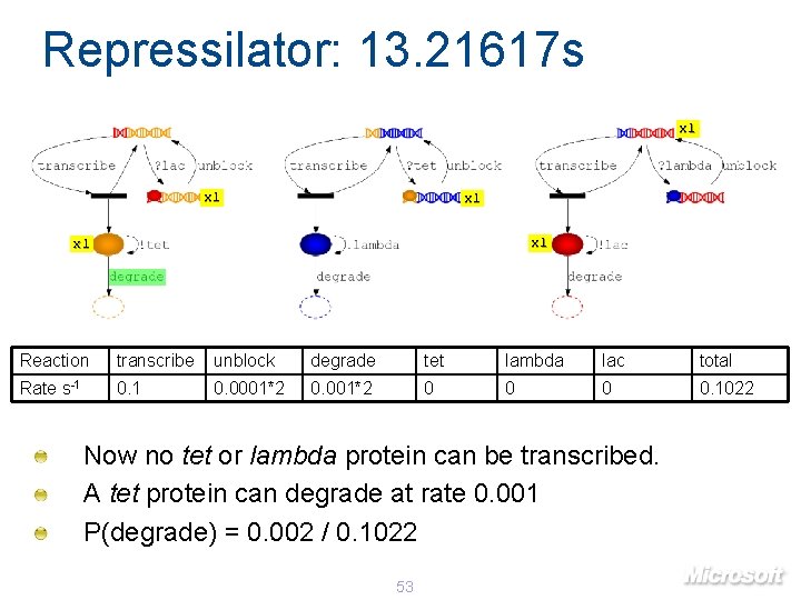
Repressilator: 13. 21617 s x 1 x 1 x 1 Reaction transcribe unblock degrade tet lambda lac total Rate s-1 0. 0001*2 0 0. 1022 Now no tet or lambda protein can be transcribed. A tet protein can degrade at rate 0. 001 P(degrade) = 0. 002 / 0. 1022 53

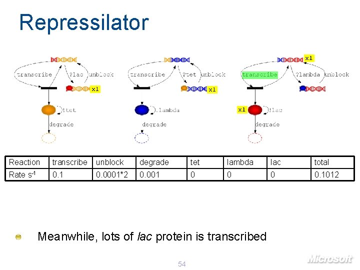
Repressilator x 1 x 1 Reaction transcribe unblock degrade tet lambda lac total Rate s-1 0. 0001*2 0. 001 0 0. 1012 Meanwhile, lots of lac protein is transcribed 54

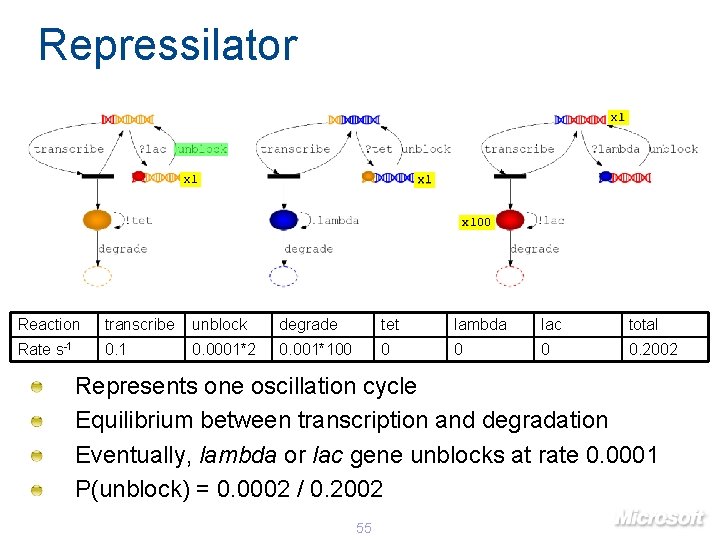
Repressilator x 1 x 100 Reaction transcribe unblock degrade tet lambda lac total Rate s-1 0. 0001*2 0. 001*100 0 0. 2002 Represents one oscillation cycle Equilibrium between transcription and degradation Eventually, lambda or lac gene unblocks at rate 0. 0001 P(unblock) = 0. 0002 / 0. 2002 55

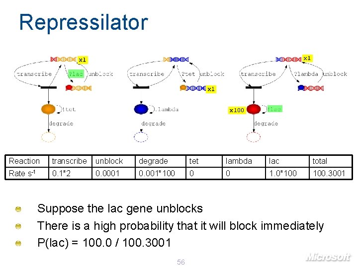
Repressilator x 1 x 100 Reaction transcribe unblock degrade tet lambda lac total Rate s-1 0. 1*2 0. 0001 0. 001*100 0 0 1. 0*100 100. 3001 Suppose the lac gene unblocks There is a high probability that it will block immediately P(lac) = 100. 0 / 100. 3001 56

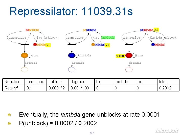
Repressilator: 11039. 31 s x 1 x 100 Reaction transcribe unblock degrade tet lambda lac total Rate s-1 0. 0001*2 0. 001*100 0 0. 2002 Eventually, the lambda gene unblocks at rate 0. 0001 P(unblock) = 0. 0002 / 0. 2002 57

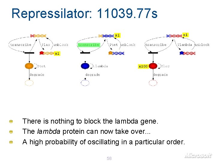
Repressilator: 11039. 77 s x 1 x 100 There is nothing to block the lambda gene. The lambda protein can now take over. . . A high probability of oscillating in a particular order. 58

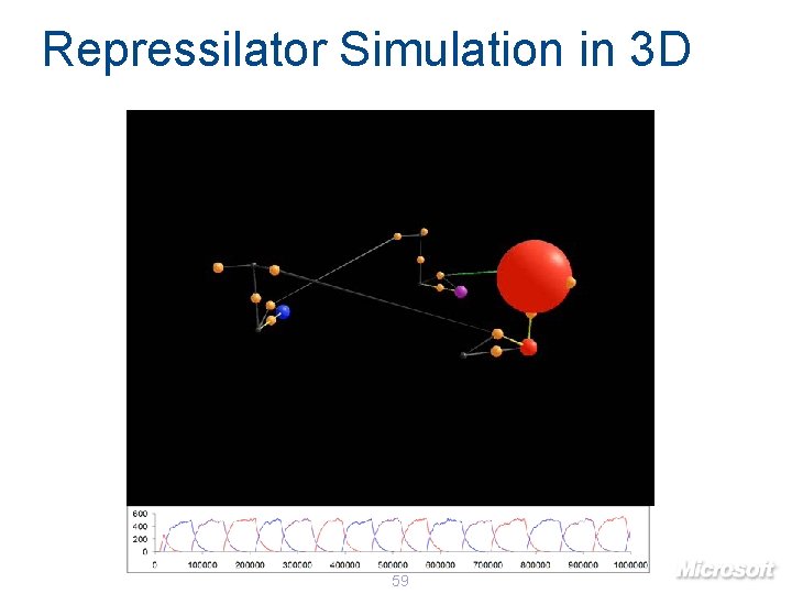
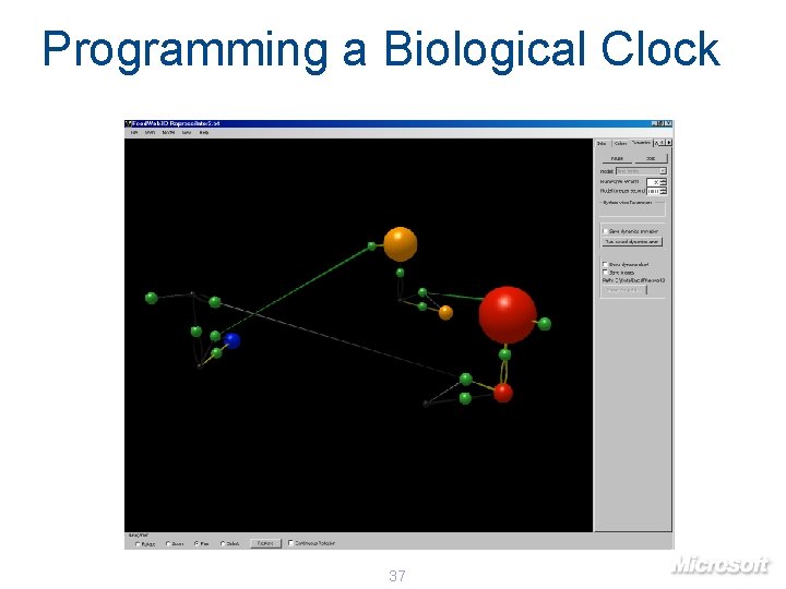
Repressilator Simulation in 3 D 59

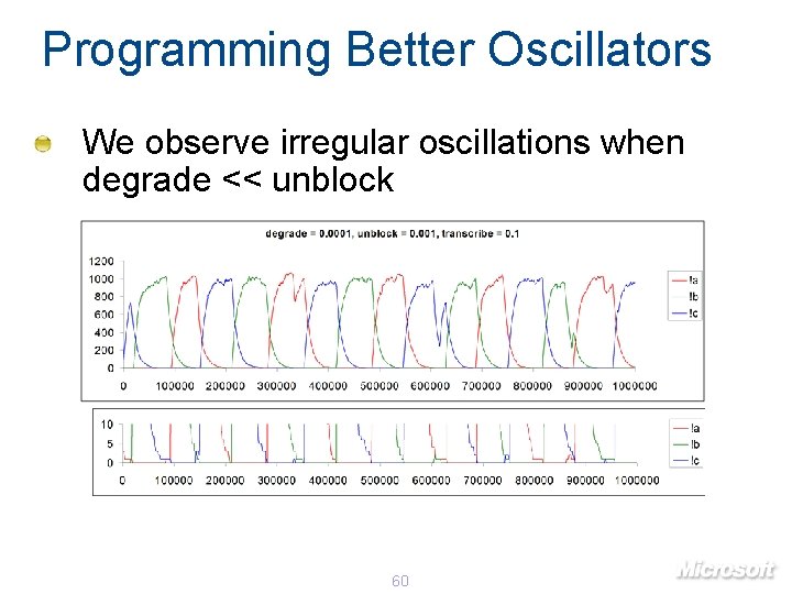
Programming Better Oscillators We observe irregular oscillations when degrade << unblock 60

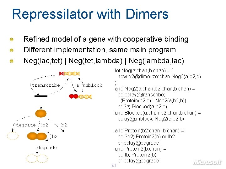
Repressilator with Dimers Refined model of a gene with cooperative binding Different implementation, same main program Neg(lac, tet) | Neg(tet, lambda) | Neg(lambda, lac) let Neg(a: chan, b: chan) = ( new b 2@dimerize: chan Neg 2(a, b 2, b) ) and Neg 2(a: chan, b 2: chan, b: chan) = do delay@transcribe; (Protein(b 2, b) | Neg 2(a, b 2, b)) or ? a; Blocked(a, b 2, b) and Blocked(a: chan, b 2: chan, b: chan) = delay@unblock; Neg 2(a, b 2, b) and Protein(b 2: chan, b: chan) = do ? b 2; Protein 2(b) or !b 2 or delay@degrade and Protein 2(b: chan) = do !b; Protein 2(b) or delay@degrade 61

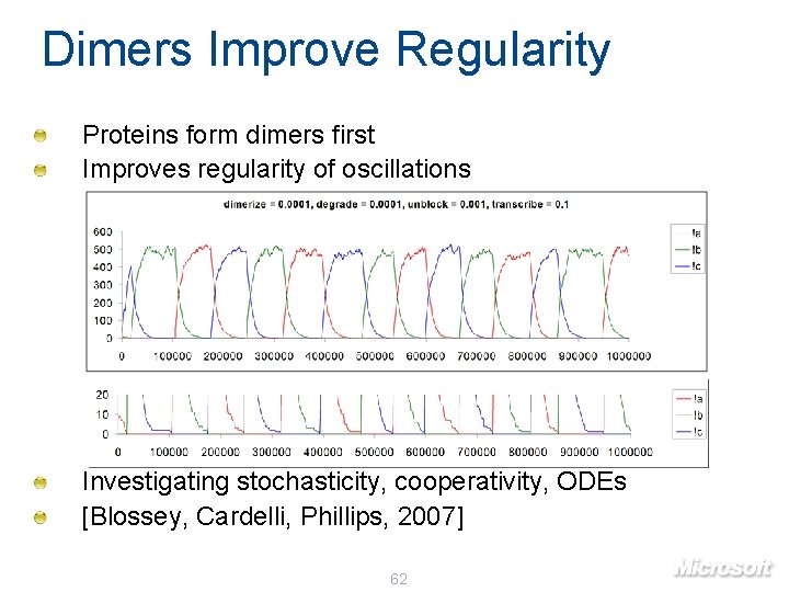
Dimers Improve Regularity Proteins form dimers first Improves regularity of oscillations Investigating stochasticity, cooperativity, ODEs [Blossey, Cardelli, Phillips, 2007] 62

Bacteria Logic Gates [Guet et al. , 2002] © 2002 AAAS. Reprinted with permission from Guet et al. Combinatorial Synthesis of Genetic Networks. Science 296 (5572): 1466 - 1470 3 genes: tet. R, lac. I, lc. I 5 promoters: PL 1, PL 2, PT, Pl-, Pl+ 125 possible networks consisting of 3 promoter-gene units 2 inputs: IPTG (represses Lac), a. Tc (represses Tet) 1 output: GFP (linked to Pl-) 63

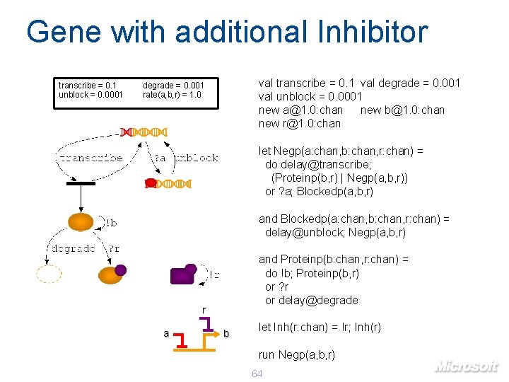
Gene with additional Inhibitor transcribe = 0. 1 unblock = 0. 0001 val transcribe = 0. 1 val degrade = 0. 001 val unblock = 0. 0001 new a@1. 0: chan new b@1. 0: chan new r@1. 0: chan degrade = 0. 001 rate(a, b, r) = 1. 0 let Negp(a: chan, b: chan, r: chan) = do delay@transcribe; (Proteinp(b, r) | Negp(a, b, r)) or ? a; Blockedp(a, b, r) and Blockedp(a: chan, b: chan, r: chan) = delay@unblock; Negp(a, b, r) and Proteinp(b: chan, r: chan) = do !b; Proteinp(b, r) or ? r or delay@degrade r a b let Inh(r: chan) = !r; Inh(r) run Negp(a, b, r) 64

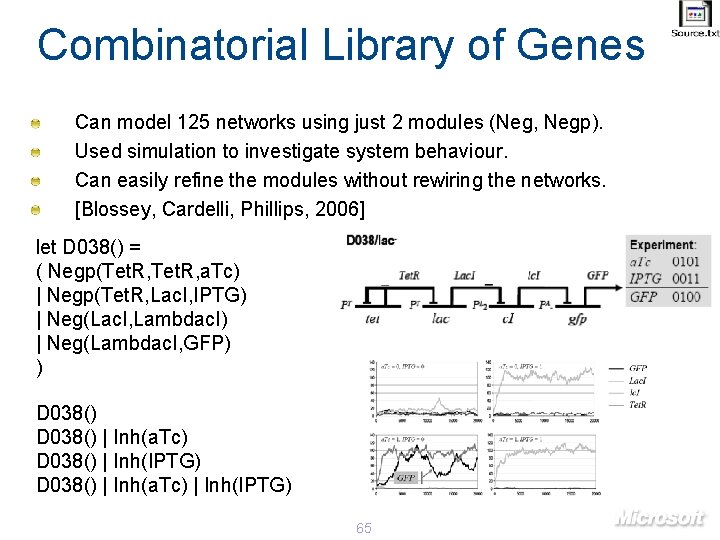
Combinatorial Library of Genes Can model 125 networks using just 2 modules (Neg, Negp). Used simulation to investigate system behaviour. Can easily refine the modules without rewiring the networks. [Blossey, Cardelli, Phillips, 2006] let D 038() = ( Negp(Tet. R, a. Tc) | Negp(Tet. R, Lac. I, IPTG) | Neg(Lac. I, Lambdac. I) | Neg(Lambdac. I, GFP) ) D 038() | Inh(a. Tc) D 038() | Inh(IPTG) D 038() | Inh(a. Tc) | Inh(IPTG) 65

Programming our Immune System with Luca Cardelli (MSR Cambridge) Leonard Goldstein (Cambridge University) Tim Elliott (Southampton University) Joern Werner (Southampton University)

MHC: A Biological Virus Scanner © 2005 from Immunobiology, Sixth Edition by Janeway et

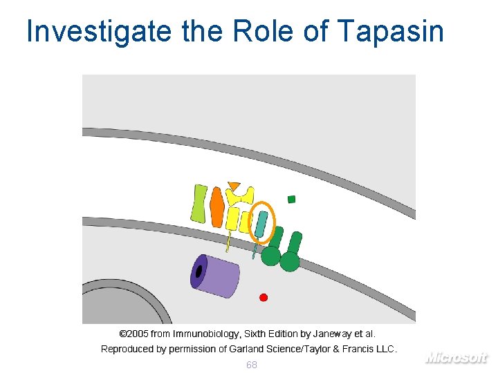
Investigate the Role of Tapasin © 2005 from Immunobiology, Sixth Edition by Janeway et

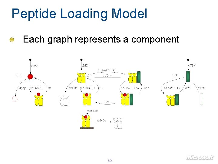
Peptide Loading Model Each graph represents a component 69

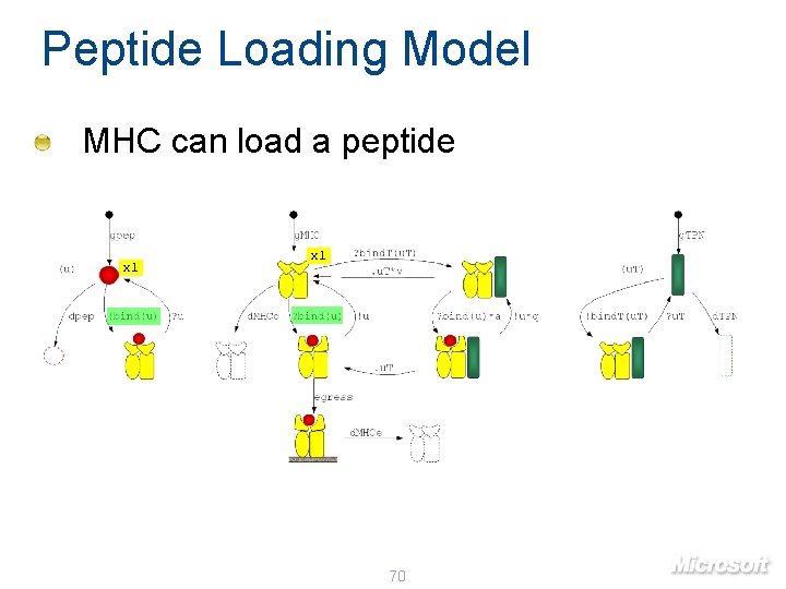
Peptide Loading Model MHC can load a peptide x 1 70

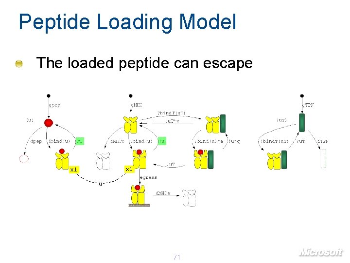
Peptide Loading Model The loaded peptide can escape x 1 u 71

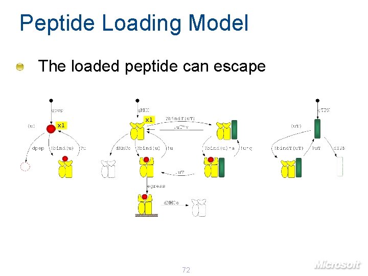
Peptide Loading Model The loaded peptide can escape x 1 72

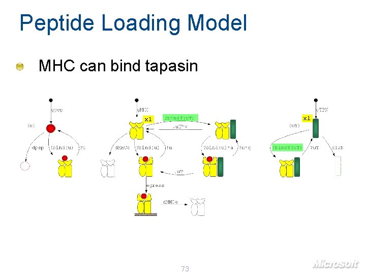
Peptide Loading Model MHC can bind tapasin x 1 73

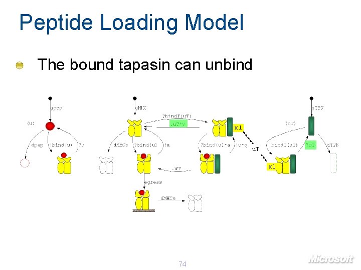
Peptide Loading Model The bound tapasin can unbind x 1 u. T x 1 74

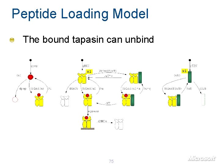
Peptide Loading Model The bound tapasin can unbind x 1 75

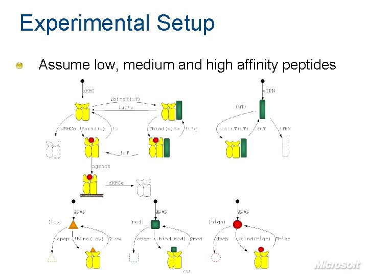
Experimental Setup Assume low, medium and high affinity peptides 76

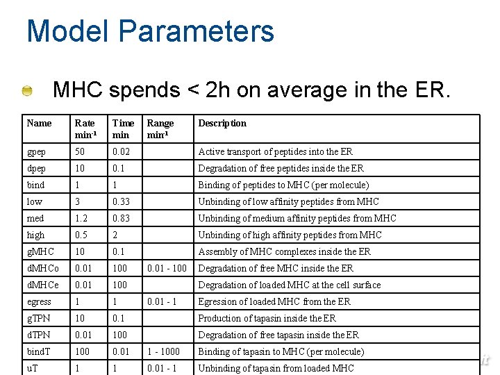
Model Parameters MHC spends < 2 h on average in the ER. Name Rate min-1 Time min Range min-1 gpep 50 0. 02 Active transport of peptides into the ER dpep 10 0. 1 Degradation of free peptides inside the ER bind 1 1 Binding of peptides to MHC (per molecule) low 3 0. 33 Unbinding of low affinity peptides from MHC med 1. 2 0. 83 Unbinding of medium affinity peptides from MHC high 0. 5 2 Unbinding of high affinity peptides from MHC g. MHC 10 0. 1 Assembly of MHC complexes inside the ER d. MHCo 0. 01 100 d. MHCe 0. 01 100 egress 1 1 g. TPN 10 0. 1 Production of tapasin inside the ER d. TPN 0. 01 100 Degradation of free tapasin inside the ER bind. T 100 0. 01 1 - 1000 Binding of tapasin to MHC (per molecule) u. T 1 1 0. 01 - 1 Unbinding of 77 tapasin from loaded MHC 0. 01 - 100 Description Degradation of free MHC inside the ER Degradation of loaded MHC at the cell surface 0. 01 - 1 Egression of loaded MHC from the ER

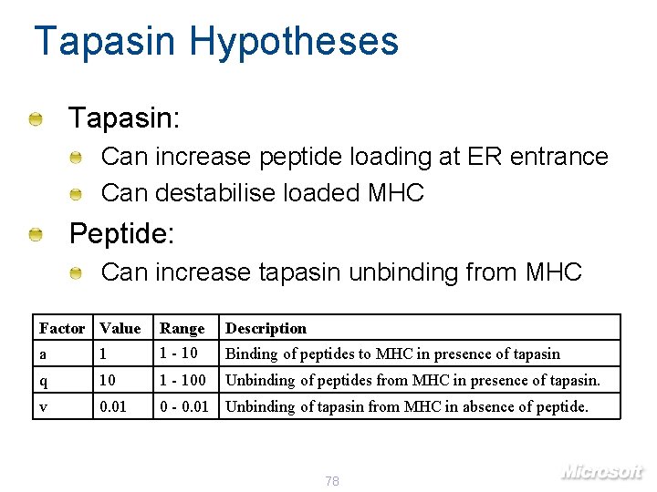
Tapasin Hypotheses Tapasin: Can increase peptide loading at ER entrance Can destabilise loaded MHC Peptide: Can increase tapasin unbinding from MHC Factor Value Range Description a 1 1 - 10 Binding of peptides to MHC in presence of tapasin q 10 1 - 100 Unbinding of peptides from MHC in presence of tapasin. v 0. 01 0 - 0. 01 Unbinding of tapasin from MHC in absence of peptide. 78

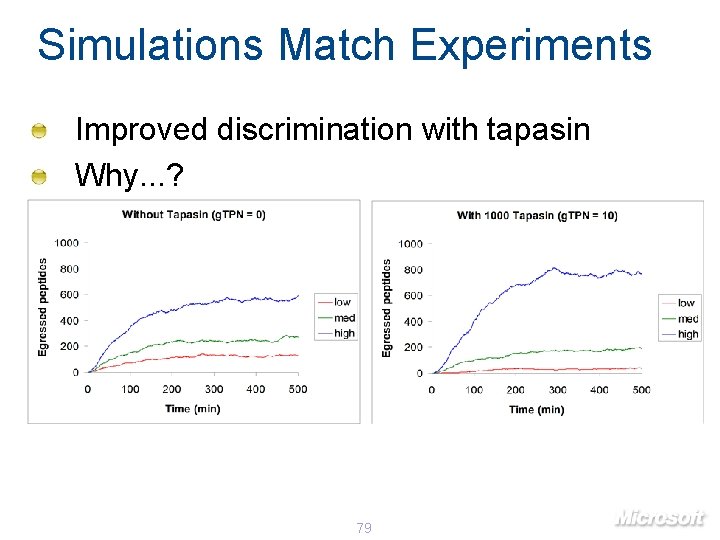
Simulations Match Experiments Improved discrimination with tapasin Why. . . ? 79

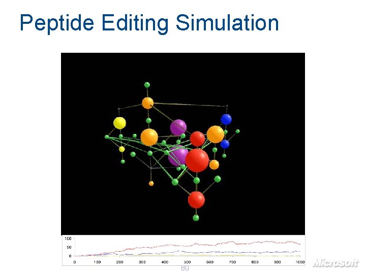
Peptide Editing Simulation 80

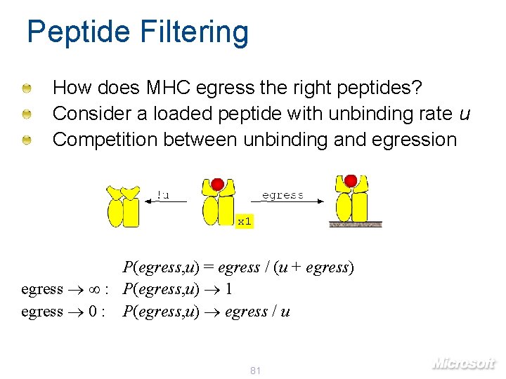
Peptide Filtering How does MHC egress the right peptides? Consider a loaded peptide with unbinding rate u Competition between unbinding and egression x 1 P(egress, u) = egress / (u + egress) egress : P(egress, u) 1 egress 0 : P(egress, u) egress / u 81

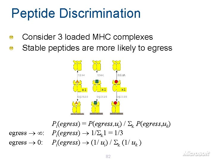
Peptide Discrimination Consider 3 loaded MHC complexes Stable peptides are more likely to egress x 1 egress : egress 0: x 1 Pi(egress) = P(egress, ui) / k P(egress, uk) Pi(egress) 1/ k 1 = 1/3 Pi(egress) (1/ ui) / k (1/ uk ) 82

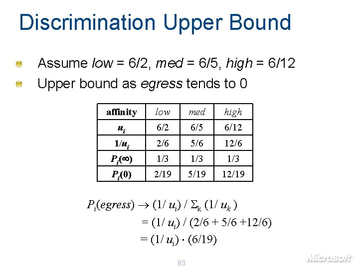
Discrimination Upper Bound Assume low = 6/2, med = 6/5, high = 6/12 Upper bound as egress tends to 0 affinity low med high ui 6/2 6/5 6/12 1/ui 2/6 5/6 12/6 Pi( ) 1/3 1/3 Pi(0) 2/19 5/19 12/19 Pi(egress) (1/ ui) / k (1/ uk ) = (1/ ui) / (2/6 + 5/6 +12/6) = (1/ ui) (6/19) 83

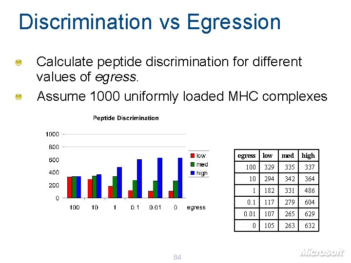
Discrimination vs Egression Calculate peptide discrimination for different values of egress. Assume 1000 uniformly loaded MHC complexes 84 egress low med high 100 329 335 337 10 294 342 364 1 182 331 486 0. 1 117 279 604 0. 01 107 265 629 0 105 263 632

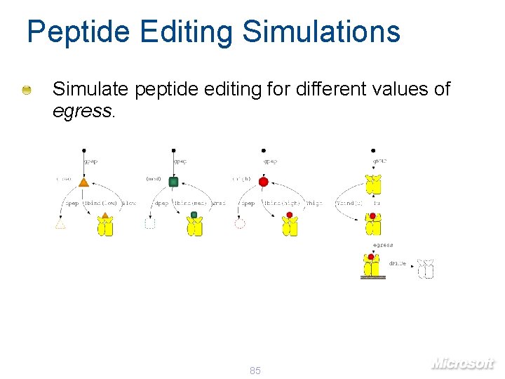
Peptide Editing Simulations Simulate peptide editing for different values of egress. 85

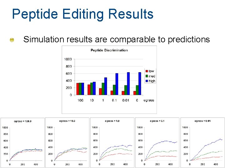
Peptide Editing Results Simulation results are comparable to predictions 86

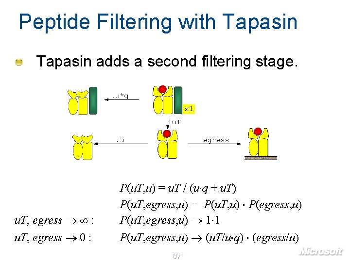
Peptide Filtering with Tapasin adds a second filtering stage. x 1 u. T, egress : P(u. T, u) = u. T / (u q + u. T) P(u. T, egress, u) = P(u. T, u) P(egress, u) P(u. T, egress, u) 1 1 u. T, egress 0 : P(u. T, egress, u) (u. T/u q) (egress/u) 87

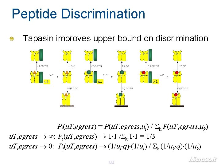
Peptide Discrimination Tapasin improves upper bound on discrimination x 1 x 1 Pi(u. T, egress) = P(u. T, egress, ui) / k P(u. T, egress, uk) u. T, egress : Pi(u. T, egress) 1 1 / k 1 1 = 1/3 u. T, egress 0: Pi(u. T, egress) (1/ui q) (1/ui) / k (1/uk q) (1/uk) 88

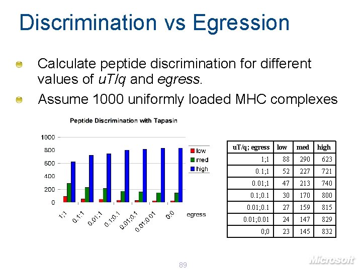
Discrimination vs Egression Calculate peptide discrimination for different values of u. T/q and egress. Assume 1000 uniformly loaded MHC complexes 89 u. T/q; egress low med high 1; 1 88 290 623 0. 1; 1 52 227 721 0. 01; 1 47 213 740 0. 1; 0. 1 30 170 800 0. 01; 0. 1 27 159 815 0. 01; 0. 01 24 147 829 0; 0 23 145 832

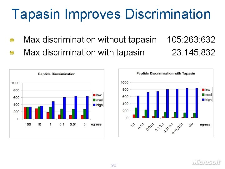
Tapasin Improves Discrimination Max discrimination without tapasin Max discrimination with tapasin 90 105: 263: 632 23: 145: 832

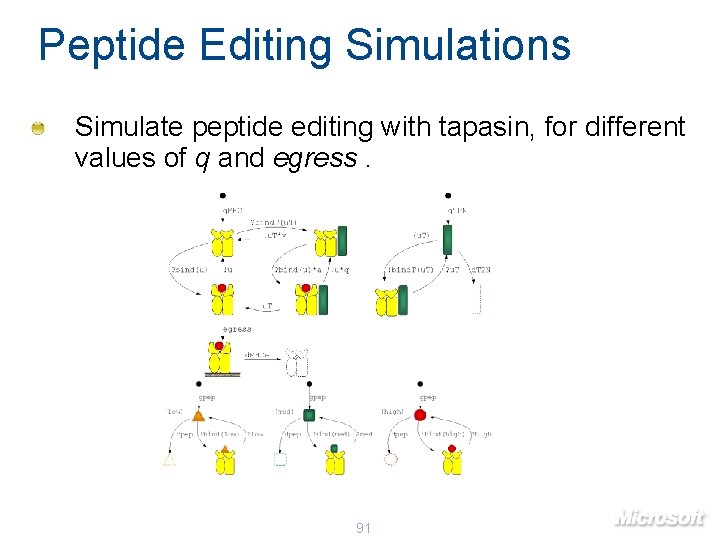
Peptide Editing Simulations Simulate peptide editing with tapasin, for different values of q and egress. 91

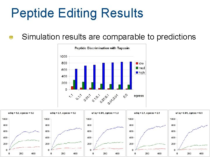
Peptide Editing Results Simulation results are comparable to predictions 92

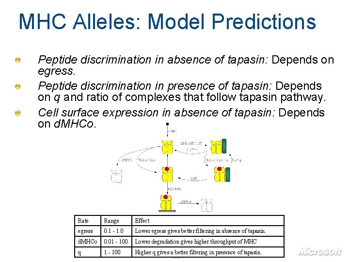
MHC Alleles: Model Predictions Peptide discrimination in absence of tapasin: Depends on egress. Peptide discrimination in presence of tapasin: Depends on q and ratio of complexes that follow tapasin pathway. Cell surface expression in absence of tapasin: Depends on d. MHCo. Rate Range Effect egress 0. 1 - 1. 0 Lower egress gives better filtering in absence of tapasin. d. MHCo 0. 01 - 100 Lower degradation gives higher throughput of MHC q 1 - 100 Higher q gives a better filtering in presence of tapasin. 93

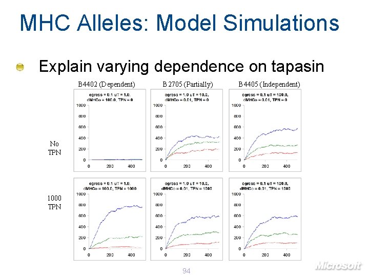
MHC Alleles: Model Simulations Explain varying dependence on tapasin B 4402 (Dependent) B 2705 (Partially) No TPN 1000 TPN 94 B 4405 (Independent)

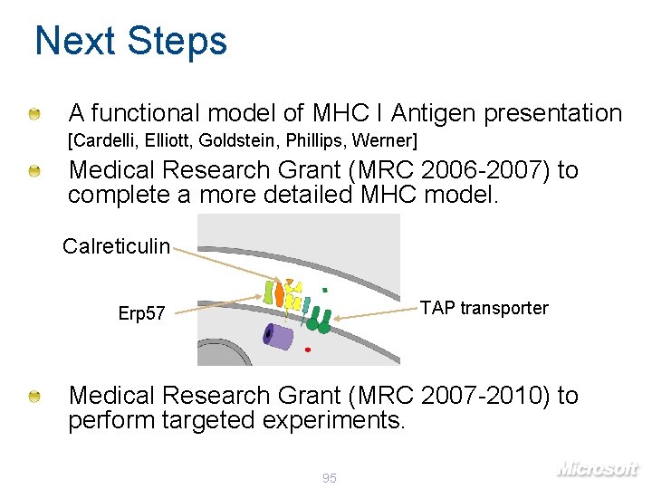
Next Steps A functional model of MHC I Antigen presentation [Cardelli, Elliott, Goldstein, Phillips, Werner] Medical Research Grant (MRC 2006 -2007) to complete a more detailed MHC model. Calreticulin TAP transporter Erp 57 Medical Research Grant (MRC 2007 -2010) to perform targeted experiments. 95

Conclusions Biological systems work surprisingly well, though we often don’t understand why We still have a lot to learn from nature. Long-term benefits for medical research: Better understand disease. Speed up the design of a cure. Long-term benefits for computing: Write more robust concurrent / distributed programs Design and verify biological computers Smart drugs? Computers in a test tube. . . ? Biological modelling is pushing the boundaries of concurrent programming 96

Thanks. 97

References [Blossey et al. , 2006] Blossey, R. , Cardelli, L. , and Phillips, A. (2006). A compositional approach to the stochastic dynamics of gene networks. Transactions in Computational Systems Biology, 3939: 99– 122. [Gillespie, 1977] Gillespie, D. T. (1977). Exact stochastic simulation of coupled chemical reactions. J. Phys. Chem. , 81(25): 2340– 2361. [Guet et al. , 2002] Guet, C. C. , Elowitz, M. B. , Hsing, W. & Leibler, S. (2002) Combinatorial synthesis of genetic networks. Science 296 1466 -1470. [Huang and Ferrel, 1996] Huang, C. -Y. F. and Ferrel, J. E. (1996). Ultrasensitivity of the mitogen-activated protein kinase cascade. PNAS, 93: 10078– 10083. [Lecca and Priami, 2003] Lecca, P. and Priami, C. (2003). Cell cycle control in eukaryotes: a biospi model. In Bio. Concur’ 03. ENTCS. [Phillips, 2006] Phillips, A. (2006). The Stochastic Pi-Machine: A Simulator for the Stochastic Pi-calculus. Available from http: //research. microsoft. com/˜aphillip/spim/. [Phillips and Cardelli, 2004] Phillips, A. and Cardelli, L. (2004). A correct abstract machine for the stochastic pi-calculus. In Bioconcur’ 04. ENTCS. [Phillips and Cardelli, 2005] Phillips, A. and Cardelli, L. (2005). A graphical representation for the stochastic pi-calculus. In Bioconcur’ 05. 98

References [Phillips et al. , 2006] Phillips, A. , Cardelli, L. , and Castagna, G. (2006). A graphical representation for biological processes in the stochastic pi-calculus. Transactions in Computational Systems Biology, 4230: 123– 152. [Priami, 1995] Priami, C. (1995). Stochastic p-calculus. The Computer Journal, 38(6): 578– 589. Proceedings of PAPM’ 95. [Priami et al. , 2001] Priami, C. , Regev, A. , Shapiro, E. , and Silverman, W. (2001). Application of a stochastic name-passing calculus to representation and simulation of molecular processes. Information Processing Letters, 80: 25– 31. [Regev et al. , 2001] Regev, A. , Silverman, W. , and Shapiro, E. (2001). Representation and simulation of biochemical processes using the pi- calculus process algebra. In Altman, R. B. , Dunker, A. K. , Hunter, L. , and Klein, T. E. , editors, Pacific Symposium on Biocomputing, volume 6, pages 459– 470, Singapore. World Scientific Press. [Sangiorgi and Walker, 2001] Sangiorgi, D. and Walker, D. (2001). The �-calculus Theory of Mobile Processes. Cambridge University Press. [Silverman et al. , 1987] Silverman, W. , Hirsch, M. , Houri, A. , and Shapiro, E. (1987). The logix system user manual, version 1. 21. In Shapiro, E. , editor, Concurrent Prolog: Collected Papers (Volume II), pages 46– 77. MIT Press, London. 99