Program Performance Asymptotic Notations CSE POSTECH Program Performance

Program Performance & Asymptotic Notations CSE, POSTECH

Program Performance l Program performance is the amount of computer memory and time needed to run a program. l How is it determined? 1. Analytically l 2. performance analysis Experimentally l performance measurement

Criteria for Measurement l Space – – l amount of memory program occupies usually measured in bytes, KB or MB Time – – execution time usually measured by the number of executions

Space Complexity l Space complexity is defined as the amount of memory a program needs to run to completion. l Why is this of concern? – – We could be running on a multi-user system where programs are allocated a specific amount of space. We may not have sufficient memory on our computer. There may be multiple solutions, each having different space requirements. The space complexity may define an upper bound on the data that the program can handle.

Components of Program Space l Program space = Instruction space + data space + stack space l The instruction space is dependent on several factors. – – the compiler that generates the machine code the compiler options that were set at compilation time the target computer See Figure 2. 1 – which one takes the least amount of instruction space?

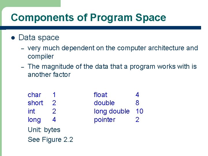
Components of Program Space l Data space – – very much dependent on the computer architecture and compiler The magnitude of the data that a program works with is another factor char 1 short 2 int 2 long 4 Unit: bytes See Figure 2. 2 float double long double pointer 4 8 10 2

Components of Program Space l Data space – – – Choosing a “smaller” data type has an effect on the overall space usage of the program. Choosing the correct type is especially important when working with arrays. How many bytes of memory are allocated with each of the following declarations? double a[100]; int maze[rows][cols];

Components of Program Space l Environment Stack Space – Every time a function is called, the following data are saved on the stack. 1. 2. 3. – the return address the values of all local variables and value formal parameters the binding of all reference and const reference parameters What is the impact of recursive function calls on the environment stack space?

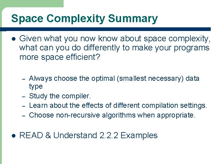
Space Complexity Summary l Given what you now know about space complexity, what can you do differently to make your programs more space efficient? – – l Always choose the optimal (smallest necessary) data type Study the compiler. Learn about the effects of different compilation settings. Choose non-recursive algorithms when appropriate. READ & Understand 2. 2. 2 Examples

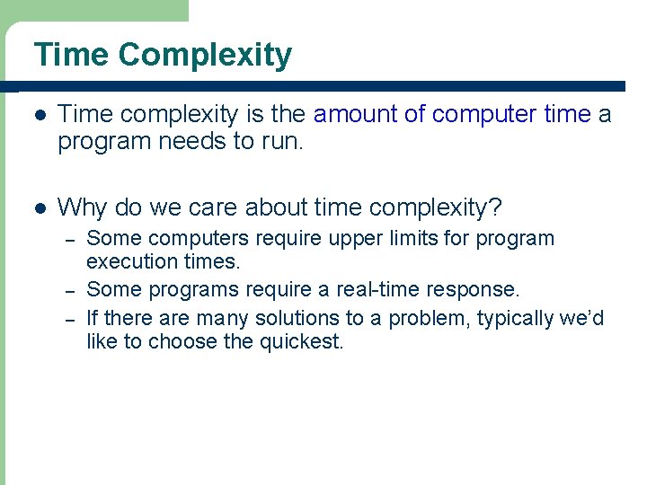
Time Complexity l Time complexity is the amount of computer time a program needs to run. l Why do we care about time complexity? – – – Some computers require upper limits for program execution times. Some programs require a real-time response. If there are many solutions to a problem, typically we’d like to choose the quickest.

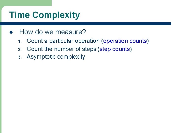
Time Complexity l How do we measure? 1. 2. 3. Count a particular operation (operation counts) Count the number of steps (step counts) Asymptotic complexity

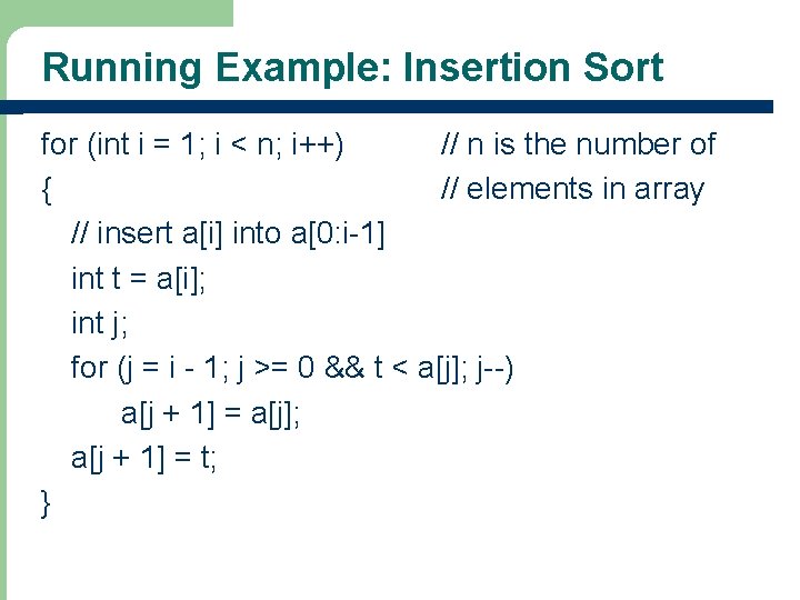
Running Example: Insertion Sort for (int i = 1; i < n; i++) // n is the number of { // elements in array // insert a[i] into a[0: i-1] int t = a[i]; int j; for (j = i - 1; j >= 0 && t < a[j]; j--) a[j + 1] = a[j]; a[j + 1] = t; }

Operation Count - Comparison for (int i = 1; i < n; i++) { // insert a[i] into a[0: i-1] int t = a[i]; int j; for (j = i - 1; j >= 0 && t < a[j]; j--) a[j + 1] = a[j]; a[j + 1] = t; }

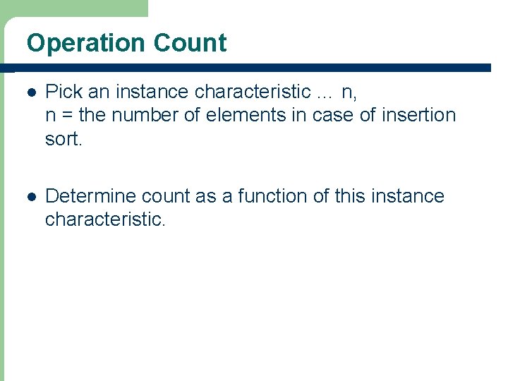
Operation Count l Pick an instance characteristic … n, n = the number of elements in case of insertion sort. l Determine count as a function of this instance characteristic.

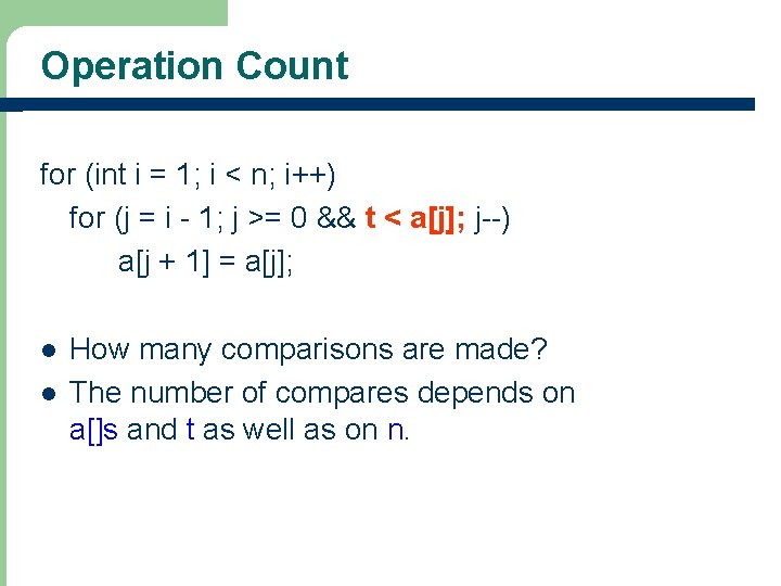
Operation Count for (int i = 1; i < n; i++) for (j = i - 1; j >= 0 && t < a[j]; j--) a[j + 1] = a[j]; l l How many comparisons are made? The number of compares depends on a[]s and t as well as on n.

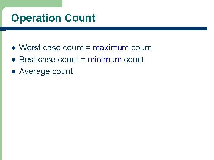
Operation Count l l l Worst case count = maximum count Best case count = minimum count Average count

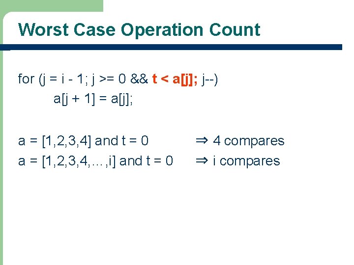
Worst Case Operation Count for (j = i - 1; j >= 0 && t < a[j]; j--) a[j + 1] = a[j]; a = [1, 2, 3, 4] and t = 0 a = [1, 2, 3, 4, …, i] and t = 0 ⇒ 4 compares ⇒ i compares

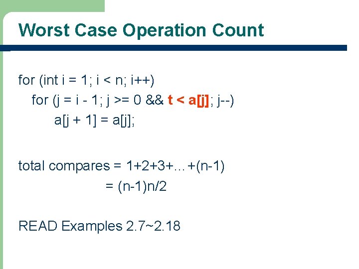
Worst Case Operation Count for (int i = 1; i < n; i++) for (j = i - 1; j >= 0 && t < a[j]; j--) a[j + 1] = a[j]; total compares = 1+2+3+…+(n-1) = (n-1)n/2 READ Examples 2. 7~2. 18

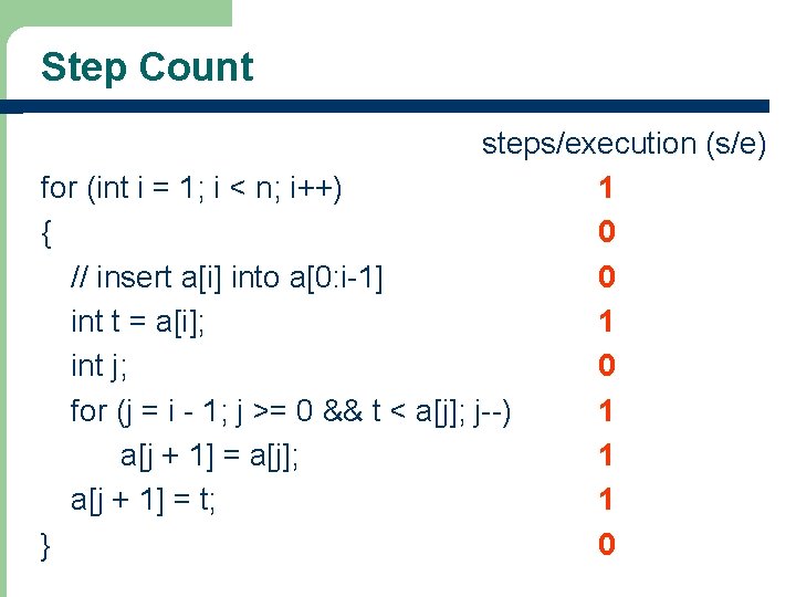
Step Count l l l The operation-count method omits accounting for the time spent on all but the chosen operation The step-count method count for all the time spent in all parts of the program A program step is loosely defined to be a syntactically or semantically meaningful segment of a program for which the execution time is independent of the instance characteristics. – – 100 adds, 100 subtracts, 1000 multiples can be counted as one step. However, n adds cannot be counted as one step.

Step Count steps/execution (s/e) for (int i = 1; i < n; i++) 1 { 0 // insert a[i] into a[0: i-1] 0 int t = a[i]; 1 int j; 0 for (j = i - 1; j >= 0 && t < a[j]; j--) 1 a[j + 1] = a[j]; 1 a[j + 1] = t; 1 } 0

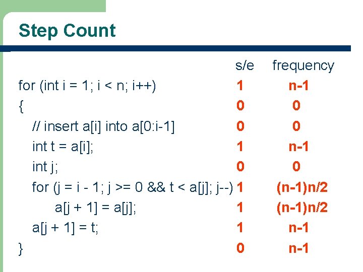
Step Count s/e for (int i = 1; i < n; i++) 1 { 0 // insert a[i] into a[0: i-1] 0 int t = a[i]; 1 int j; 0 for (j = i - 1; j >= 0 && t < a[j]; j--) 1 a[j + 1] = a[j]; 1 a[j + 1] = t; 1 } 0 frequency n-1 0 0 n-1 0 (n-1)n/2 n-1

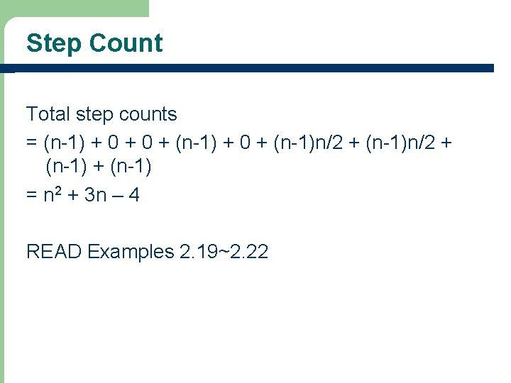
Step Count Total step counts = (n-1) + 0 + (n-1)n/2 + (n-1) = n 2 + 3 n – 4 READ Examples 2. 19~2. 22

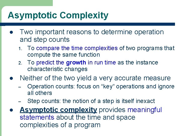
Asymptotic Complexity l Two important reasons to determine operation and step counts 1. 2. l Neither of the two yield a very accurate measure – – l To compare the time complexities of two programs that compute the same function To predict the growth in run time as the instance characteristic changes Operation counts: focus on “key” operations and ignore all others Step counts: the notion of a step is itself inexact Asymptotic complexity provides meaningful statements about the time and space complexities of a program

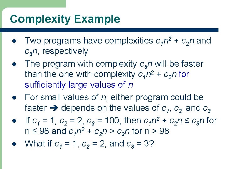
Complexity Example l l l Two programs have complexities c 1 n 2 + c 2 n and c 3 n, respectively The program with complexity c 3 n will be faster than the one with complexity c 1 n 2 + c 2 n for sufficiently large values of n For small values of n, either program could be faster depends on the values of c 1, c 2 and c 3 If c 1 = 1, c 2 = 2, c 3 = 100, then c 1 n 2 + c 2 n ≤ c 3 n for n ≤ 98 and c 1 n 2 + c 2 n > c 3 n for n > 98 What if c 1 = 1, c 2 = 2, and c 3 = 3?

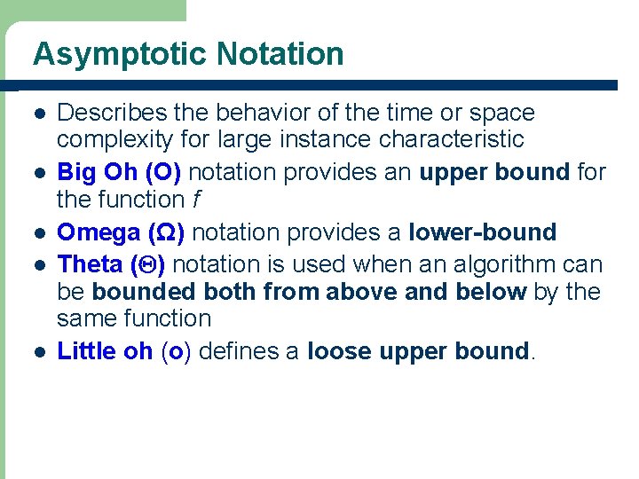
Asymptotic Notation l l l Describes the behavior of the time or space complexity for large instance characteristic Big Oh (O) notation provides an upper bound for the function f Omega (Ω) notation provides a lower-bound Theta (Q) notation is used when an algorithm can be bounded both from above and below by the same function Little oh (o) defines a loose upper bound.

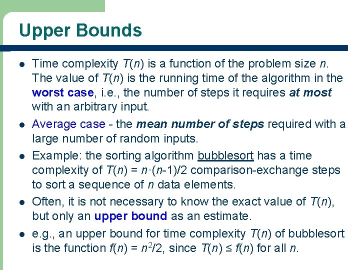
Upper Bounds l l l Time complexity T(n) is a function of the problem size n. The value of T(n) is the running time of the algorithm in the worst case, i. e. , the number of steps it requires at most with an arbitrary input. Average case - the mean number of steps required with a large number of random inputs. Example: the sorting algorithm bubblesort has a time complexity of T(n) = n·(n-1)/2 comparison-exchange steps to sort a sequence of n data elements. Often, it is not necessary to know the exact value of T(n), but only an upper bound as an estimate. e. g. , an upper bound for time complexity T(n) of bubblesort is the function f(n) = n 2/2, since T(n) ≤ f(n) for all n.

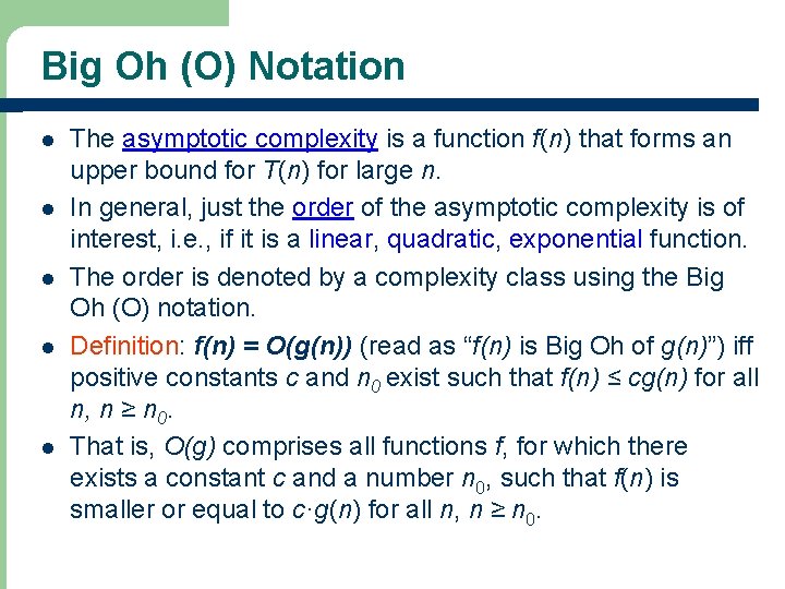
Big Oh (O) Notation l l l The asymptotic complexity is a function f(n) that forms an upper bound for T(n) for large n. In general, just the order of the asymptotic complexity is of interest, i. e. , if it is a linear, quadratic, exponential function. The order is denoted by a complexity class using the Big Oh (O) notation. Definition: f(n) = O(g(n)) (read as “f(n) is Big Oh of g(n)”) iff positive constants c and n 0 exist such that f(n) ≤ cg(n) for all n, n ≥ n 0. That is, O(g) comprises all functions f, for which there exists a constant c and a number n 0, such that f(n) is smaller or equal to c·g(n) for all n, n ≥ n 0.

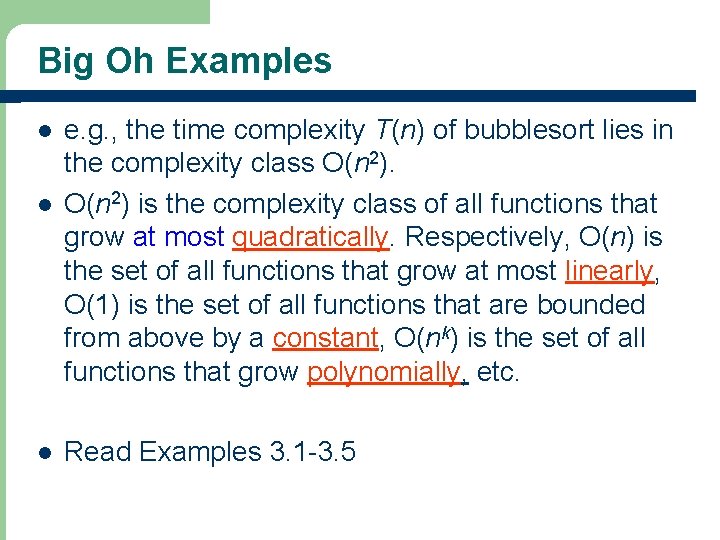
Big Oh Examples l l l e. g. , the time complexity T(n) of bubblesort lies in the complexity class O(n 2) is the complexity class of all functions that grow at most quadratically. Respectively, O(n) is the set of all functions that grow at most linearly, O(1) is the set of all functions that are bounded from above by a constant, O(nk) is the set of all functions that grow polynomially, etc. Read Examples 3. 1 -3. 5

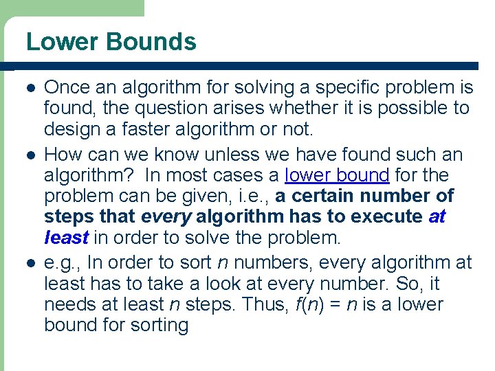
Lower Bounds l l l Once an algorithm for solving a specific problem is found, the question arises whether it is possible to design a faster algorithm or not. How can we know unless we have found such an algorithm? In most cases a lower bound for the problem can be given, i. e. , a certain number of steps that every algorithm has to execute at least in order to solve the problem. e. g. , In order to sort n numbers, every algorithm at least has to take a look at every number. So, it needs at least n steps. Thus, f(n) = n is a lower bound for sorting

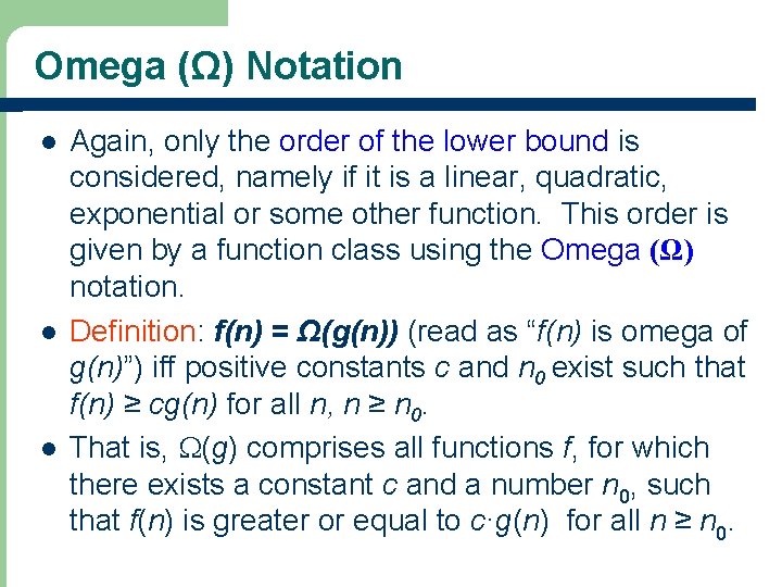
Omega (Ω) Notation l l l Again, only the order of the lower bound is considered, namely if it is a linear, quadratic, exponential or some other function. This order is given by a function class using the Omega (Ω) notation. Definition: f(n) = Ω(g(n)) (read as “f(n) is omega of g(n)”) iff positive constants c and n 0 exist such that f(n) ≥ cg(n) for all n, n ≥ n 0. That is, W(g) comprises all functions f, for which there exists a constant c and a number n 0, such that f(n) is greater or equal to c·g(n) for all n ≥ n 0.

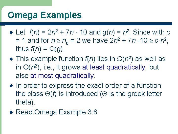
Omega Examples l l Let f(n) = 2 n 2 + 7 n - 10 and g(n) = n 2. Since with c = 1 and for n ≥ n 0 = 2 we have 2 n 2 + 7 n -10 ≥ c·n 2, thus f(n) = W(g). This example function f(n) lies in W(n 2) as well as in O(n 2), i. e. , it grows at least quadratically, but also at most quadratically. In order to express the exact order of a function the class Q(f) is introduced (Q is the greek letter theta). Read Omega Example 3. 6

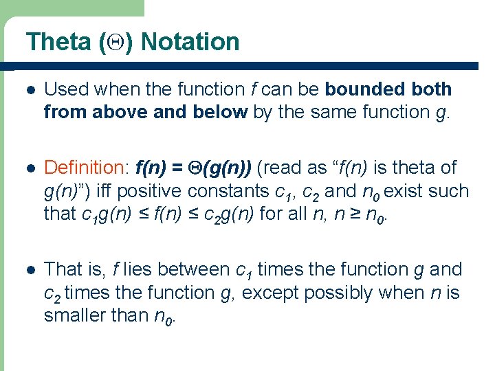
Theta (Q) Notation l Used when the function f can be bounded both from above and below by the same function g. l Definition: f(n) = Q(g(n)) (read as “f(n) is theta of g(n)”) iff positive constants c 1, c 2 and n 0 exist such that c 1 g(n) ≤ f(n) ≤ c 2 g(n) for all n, n ≥ n 0. l That is, f lies between c 1 times the function g and c 2 times the function g, except possibly when n is smaller than n 0.

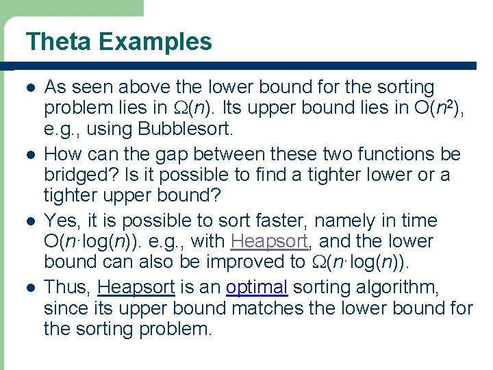
Theta Examples l l As seen above the lower bound for the sorting problem lies in W(n). Its upper bound lies in O(n 2), e. g. , using Bubblesort. How can the gap between these two functions be bridged? Is it possible to find a tighter lower or a tighter upper bound? Yes, it is possible to sort faster, namely in time O(n·log(n)). e. g. , with Heapsort, and the lower bound can also be improved to W(n·log(n)). Thus, Heapsort is an optimal sorting algorithm, since its upper bound matches the lower bound for the sorting problem.

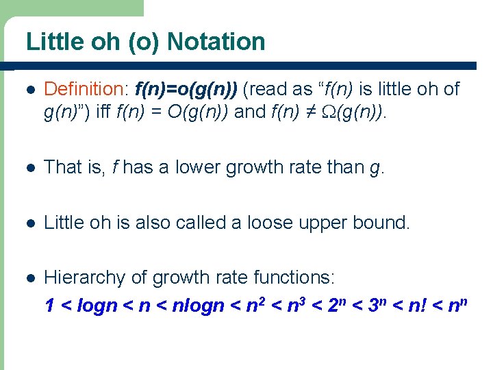
Little oh (o) Notation l Definition: f(n)=o(g(n)) (read as “f(n) is little oh of g(n)”) iff f(n) = O(g(n)) and f(n) ≠ W(g(n)). l That is, f has a lower growth rate than g. l Little oh is also called a loose upper bound. l Hierarchy of growth rate functions: 1 < logn < nlogn < n 2 < n 3 < 2 n < 3 n < n! < nn

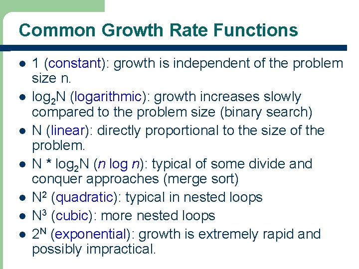
Common Growth Rate Functions l l l l 1 (constant): growth is independent of the problem size n. log 2 N (logarithmic): growth increases slowly compared to the problem size (binary search) N (linear): directly proportional to the size of the problem. N * log 2 N (n log n): typical of some divide and conquer approaches (merge sort) N 2 (quadratic): typical in nested loops N 3 (cubic): more nested loops 2 N (exponential): growth is extremely rapid and possibly impractical.

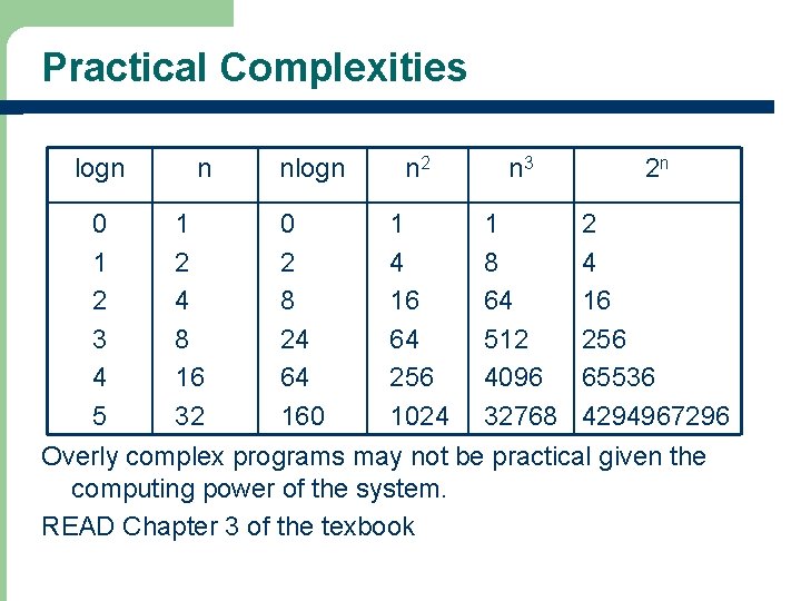
Practical Complexities logn 0 1 2 3 4 5 n 1 2 4 8 16 32 nlogn 0 2 8 24 64 160 n 2 n 3 2 n 1 4 16 64 256 1024 1 8 64 512 4096 32768 2 4 16 256 65536 4294967296 Overly complex programs may not be practical given the computing power of the system. READ Chapter 3 of the texbook