Profit Maximization Power Point Slides prepared by Andreea

Profit Maximization Power. Point Slides prepared by: Andreea CHIRITESCU Eastern Illinois University © 2012 Cengage Learning. All Rights Reserved. May not be copied, scanned, or duplicated, in whole or in part, except for use as permitted in a license distributed with a certain product or service or otherwise on a password-protected website for classroom use. 1

The Nature and Behavior of Firms • A firm – An association of individuals • Who have organized themselves for the purpose of turning inputs into outputs • Firms – All shapes and sizes – Structure of their management – Financial instruments © 2012 Cengage Learning. All Rights Reserved. May not be copied, scanned, or duplicated, in whole or in part, except for use as permitted in a license distributed with a certain product or service or otherwise on a password-protected website for classroom use. 2

The Nature and Behavior of Firms • Simple model of a firm – Technology given by the production function, f(k, l) • Inputs: labor (l) and capital (k) – Run by an entrepreneur • Makes all the decisions • Receives all the profits and losses from the firm’s operations • Acts in his or her own self-interest – Maximize the firm’s profits © 2012 Cengage Learning. All Rights Reserved. May not be copied, scanned, or duplicated, in whole or in part, except for use as permitted in a license distributed with a certain product or service or otherwise on a password-protected website for classroom use. 3

The Nature and Behavior of Firms • Complicating factors – Management team – Shareholders – Owners – Outsourcing • Firms – Are not individuals but can be much more complicated organizations – Firm’s objectives: profit maximization © 2012 Cengage Learning. All Rights Reserved. May not be copied, scanned, or duplicated, in whole or in part, except for use as permitted in a license distributed with a certain product or service or otherwise on a password-protected website for classroom use. 4

Profit Maximization • A profit-maximizing firm – Chooses both its inputs and its outputs • With the sole goal of achieving maximum economic profits – Seeks to maximize the difference between total revenue and total economic costs – Make decisions in a “marginal” way • Examine the marginal profit obtainable from producing one more unit of hiring one additional laborer © 2012 Cengage Learning. All Rights Reserved. May not be copied, scanned, or duplicated, in whole or in part, except for use as permitted in a license distributed with a certain product or service or otherwise on a password-protected website for classroom use. 5

Output Choice • Total revenue for a firm, R(q) = p(q) q • Economic costs incurred, C(q) – In the production of q • Economic profits, – The difference between total revenue and total costs (q) = R(q) – C(q) = p(q) q –C(q) © 2012 Cengage Learning. All Rights Reserved. May not be copied, scanned, or duplicated, in whole or in part, except for use as permitted in a license distributed with a certain product or service or otherwise on a password-protected website for classroom use. 6

Output Choice • The necessary condition – For choosing the level of q that maximizes profits • Setting the derivative of the function with respect to q equal to zero © 2012 Cengage Learning. All Rights Reserved. May not be copied, scanned, or duplicated, in whole or in part, except for use as permitted in a license distributed with a certain product or service or otherwise on a password-protected website for classroom use. 7

Output Choice • Marginal revenue, MR – The change in total revenue R resulting from a change in output q Marginal revenue = MR = d. R/dq • Profit maximization – Maximize economic profits – Choose output q* at which MR(q*)=MC(q*) © 2012 Cengage Learning. All Rights Reserved. May not be copied, scanned, or duplicated, in whole or in part, except for use as permitted in a license distributed with a certain product or service or otherwise on a password-protected website for classroom use. 8

Second-Order Conditions • MR = MC – Is only a necessary condition for profit maximization • For sufficiency, it is also required: • ‘‘marginal’’ profit must decrease at the optimal level of output, q* – For q<q*, ’(q) > 0 – For q>q*, ’(q) < 0 © 2012 Cengage Learning. All Rights Reserved. May not be copied, scanned, or duplicated, in whole or in part, except for use as permitted in a license distributed with a certain product or service or otherwise on a password-protected website for classroom use. 9

11. 1 (a) Marginal Revenue Must Equal Marginal Cost for Profit Maximization Revenues, Costs C R q** q* Output period Profits, defined as revenues (R) minus costs (C), reach a maximum when the slope of the revenue function (marginal revenue) is equal to the slope of the cost function (marginal cost). This equality is only a necessary condition for a maximum, as may be seen by comparing points q* (a true maximum) and q** (a local minimum), points at which marginal revenue equals marginal cost. © 2012 Cengage Learning. All Rights Reserved. May not be copied, scanned, or duplicated, in whole or in part, except for use as permitted in a license distributed with a certain product or service or otherwise on a password-protected website for classroom use. 10

11. 1 (b) Marginal Revenue Must Equal Marginal Cost for Profit Maximization Profits q* Output period Losses Profits, defined as revenues (R) minus costs (C), reach a maximum when the slope of the revenue function (marginal revenue) is equal to the slope of the cost function (marginal cost). This equality is only a necessary condition for a maximum, as may be seen by comparing points q* (a true maximum) and q** (a local minimum), points at which marginal revenue equals marginal cost. © 2012 Cengage Learning. All Rights Reserved. May not be copied, scanned, or duplicated, in whole or in part, except for use as permitted in a license distributed with a certain product or service or otherwise on a password-protected website for classroom use. 11

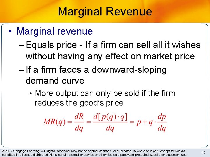
Marginal Revenue • Marginal revenue – Equals price - If a firm can sell all it wishes without having any effect on market price – If a firm faces a downward-sloping demand curve • More output can only be sold if the firm reduces the good’s price © 2012 Cengage Learning. All Rights Reserved. May not be copied, scanned, or duplicated, in whole or in part, except for use as permitted in a license distributed with a certain product or service or otherwise on a password-protected website for classroom use. 12

Marginal Revenue • Marginal revenue - is a function of output – If price does not change as quantity increases • dp/dq = 0, MR = price • The firm is a price taker – If price decreases as quantity increases • dp/dq < 0, MR < price © 2012 Cengage Learning. All Rights Reserved. May not be copied, scanned, or duplicated, in whole or in part, except for use as permitted in a license distributed with a certain product or service or otherwise on a password-protected website for classroom use. 13

11. 1 Marginal Revenue from a Linear Demand Function • Demand curve for a sub sandwich is q = 100 – 10 p • Solving for price: p = -q/10 + 10 • Total revenue: R = pq = -q 2/10 + 10 q • Marginal revenue: MR = d. R/dq = -q/5 + 10 • MR < p for all values of q • If the average and marginal costs are constant ($4) • Profit maximizing quantity: MR = MC, so q*=30 • Price = $7, and profits = $90 © 2012 Cengage Learning. All Rights Reserved. May not be copied, scanned, or duplicated, in whole or in part, except for use as permitted in a license distributed with a certain product or service or otherwise on a password-protected website for classroom use. 14

Marginal Revenue and Elasticity • Marginal revenue – Directly related to the elasticity of the demand curve facing the firm • The price elasticity of demand – Percentage change in quantity that results from a one percent change in price © 2012 Cengage Learning. All Rights Reserved. May not be copied, scanned, or duplicated, in whole or in part, except for use as permitted in a license distributed with a certain product or service or otherwise on a password-protected website for classroom use. 15

Marginal Revenue and Elasticity • This means that – If demand curve slopes downward – eq, p < 0 and MR < p – If demand is elastic: eq, p < -1 and MR > 0 – If demand is infinitely elastic: eq, p = - and MR = p – If demand is inelastic: eq, p > 1 and MR < 0 © 2012 Cengage Learning. All Rights Reserved. May not be copied, scanned, or duplicated, in whole or in part, except for use as permitted in a license distributed with a certain product or service or otherwise on a password-protected website for classroom use. 16

11. 1 Relationship between Elasticity and Marginal Revenue © 2012 Cengage Learning. All Rights Reserved. May not be copied, scanned, or duplicated, in whole or in part, except for use as permitted in a license distributed with a certain product or service or otherwise on a password-protected website for classroom use. 17

Price–Marginal Cost Markup • Maximize profits: MR = MC – If demand is downward sloping and thus eq, p < 0 – Formula for the percentage ‘‘markup’’ of price over marginal cost • This demand facing the firm must be elastic, eq, p<1 • The percentage markup over marginal cost will be higher the closer eq, p is to 1 © 2012 Cengage Learning. All Rights Reserved. May not be copied, scanned, or duplicated, in whole or in part, except for use as permitted in a license distributed with a certain product or service or otherwise on a password-protected website for classroom use. 18

Average Revenue Curve • Assume – That the firm must sell all its output at one price – So, we can think of the demand curve facing the firm as its average revenue curve • Shows the revenue per unit yielded by alternative output choices © 2012 Cengage Learning. All Rights Reserved. May not be copied, scanned, or duplicated, in whole or in part, except for use as permitted in a license distributed with a certain product or service or otherwise on a password-protected website for classroom use. 19

Marginal Revenue Curve • Marginal revenue curve – Shows the extra revenue provided by the last unit sold – Below the demand curve • In the case of a downward-sloping demand curve © 2012 Cengage Learning. All Rights Reserved. May not be copied, scanned, or duplicated, in whole or in part, except for use as permitted in a license distributed with a certain product or service or otherwise on a password-protected website for classroom use. 20

11. 2 Market Demand Curve and Associated Marginal Revenue Curve Price p 1 D (average revenue) q 1 Quantity period MR Because the demand curve is negatively sloped, the marginal revenue curve will fall below the demand (‘‘average revenue’’) curve. For output levels beyond q 1, MR is negative. At q 1, total revenues (p 1 · q 1) are a maximum; beyond this point, additional increases in q cause total revenues to decrease because of the concomitant decreases in price. © 2012 Cengage Learning. All Rights Reserved. May not be copied, scanned, or duplicated, in whole or in part, except for use as permitted in a license distributed with a certain product or service or otherwise on a password-protected website for classroom use. 21

Marginal Revenue Curve • When the demand curve shifts – The marginal revenue curve associated with it shifts as well • A marginal revenue curve – Cannot be calculated without referring to a specific demand curve © 2012 Cengage Learning. All Rights Reserved. May not be copied, scanned, or duplicated, in whole or in part, except for use as permitted in a license distributed with a certain product or service or otherwise on a password-protected website for classroom use. 22

11. 2 The Constant Elasticity Case • Demand function of the form: q = apb • Has a constant price elasticity of demand = -b • Solving this equation for p, we get p = (1/a)1/bq 1/b = kq 1/b where k = (1/a)1/b • Hence: R = pq = kq(1+b)/b • And MR = dr/dq = [(1+b)/b]kq 1/b = [(1+b)/b]p • This implies that MR is proportional to price © 2012 Cengage Learning. All Rights Reserved. May not be copied, scanned, or duplicated, in whole or in part, except for use as permitted in a license distributed with a certain product or service or otherwise on a password-protected website for classroom use. 23

Short-Run Supply by a Price-Taking Firm • Price-taking firm – Demand curve facing the firm is a horizontal line through P*=MR – Profit-maximizing output level, q* • P*= short run marginal costs • And marginal cost is increasing – At q*, profits are – Positive if price > average costs – Negative (loss) if price < average costs – Zero if price = average costs © 2012 Cengage Learning. All Rights Reserved. May not be copied, scanned, or duplicated, in whole or in part, except for use as permitted in a license distributed with a certain product or service or otherwise on a password-protected website for classroom use. 24

11. 3 Short-Run Supply Curve for a Price-Taking Firm Market price SMC P** SAC P* = MR SAVC P*** Ps q*** q* q** Quantity period In the short run, a price-taking firm will produce the level of output for which SMC =P. At P*, for example, the firm will produce q*. The SMC curve also shows what will be produced at other prices. For prices below SAVC, however, the firm will choose to produce no output. The heavy lines in the figure represent the firm’s short-run supply curve. © 2012 Cengage Learning. All Rights Reserved. May not be copied, scanned, or duplicated, in whole or in part, except for use as permitted in a license distributed with a certain product or service or otherwise on a password-protected website for classroom use. 25

Short-Run Supply by a Price-Taking Firm • Short-run supply curve – The positively-sloped portion of the shortrun marginal cost curve – Above the point of minimum average variable cost – It shows how much the firm will produce at every possible market price © 2012 Cengage Learning. All Rights Reserved. May not be copied, scanned, or duplicated, in whole or in part, except for use as permitted in a license distributed with a certain product or service or otherwise on a password-protected website for classroom use. 26

Short-Run Supply by a Price-Taking Firm • Firms will only operate in the short run – As long as total revenue covers variable cost – p > SAVC • Firms will shut-down in the short-run – If p < SAVC – Produce no output © 2012 Cengage Learning. All Rights Reserved. May not be copied, scanned, or duplicated, in whole or in part, except for use as permitted in a license distributed with a certain product or service or otherwise on a password-protected website for classroom use. 27

11. 3 Short-Run Supply • Firm’s short-run total cost curve is SC(v, w, q, k) = vk 1 + wq 1/ k 1 - / • Where k 1 is the level of capital held constant in the short run • Short-run marginal cost is • The price-taking firm will maximize profit where p = SMC © 2012 Cengage Learning. All Rights Reserved. May not be copied, scanned, or duplicated, in whole or in part, except for use as permitted in a license distributed with a certain product or service or otherwise on a password-protected website for classroom use. 28

11. 3 Short-Run Supply • Quantity supplied will be • To find the firm’s shut-down price, we need to solve for SAVC SVC = wq 1/ k 1 - / SAVC = SVC/q = wq(1 - )/ k 1 - / • SAVC < SMC for all values of < 1 • There is no price low enough that the firm will want to shut down © 2012 Cengage Learning. All Rights Reserved. May not be copied, scanned, or duplicated, in whole or in part, except for use as permitted in a license distributed with a certain product or service or otherwise on a password-protected website for classroom use. 29

Profit Functions • A firm’s economic profit can be expressed as a function of inputs = Pq - C(q) = Pf(k, l) - vk - wl – Only k and l are under the firm’s control – P, v, and w - fixed parameters • Profit function – Shows its maximal profits as a function of the prices that the firm faces © 2012 Cengage Learning. All Rights Reserved. May not be copied, scanned, or duplicated, in whole or in part, except for use as permitted in a license distributed with a certain product or service or otherwise on a password-protected website for classroom use. 30

Properties of the Profit Function • Homogeneity – The profit function is homogeneous of degree one in all prices • Nondecreasing in output price, P • Nonincreasing in input prices, v, and w • Convex in output prices © 2012 Cengage Learning. All Rights Reserved. May not be copied, scanned, or duplicated, in whole or in part, except for use as permitted in a license distributed with a certain product or service or otherwise on a password-protected website for classroom use. 31

Envelope Results • Apply the envelope theorem – To see how profits respond to changes in output and input prices © 2012 Cengage Learning. All Rights Reserved. May not be copied, scanned, or duplicated, in whole or in part, except for use as permitted in a license distributed with a certain product or service or otherwise on a password-protected website for classroom use. 32

Producer Surplus in the Short Run • Profit function is nondecreasing in output prices – If P 2 > P 1, (P 2, …) (P 1, …) – The welfare gain to the firm of from the price change: welfare gain = (P 2, …) – (P 1, …) © 2012 Cengage Learning. All Rights Reserved. May not be copied, scanned, or duplicated, in whole or in part, except for use as permitted in a license distributed with a certain product or service or otherwise on a password-protected website for classroom use. 33

11. 4 Changes in Short-Run Producer Surplus Measure Firm Profits Market price SMC P 2 A P 1 Ps B C q 1 q 2 Quantity period If price increases from P 1 to P 2, then the increase in the firm’s profits is given by area P 2 ABP 1. At a price of P 1, the firm earns short-run producer surplus given by area Ps. CBP 1. This measures the increase in short-run profits for the firm when it produces q 1 rather than shutting down when price is Ps or below. © 2012 Cengage Learning. All Rights Reserved. May not be copied, scanned, or duplicated, in whole or in part, except for use as permitted in a license distributed with a certain product or service or otherwise on a password-protected website for classroom use. 34

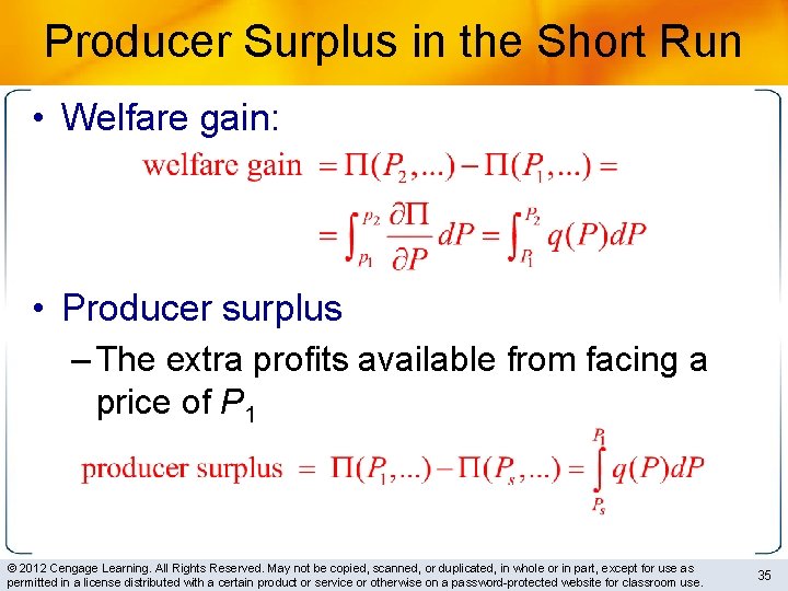
Producer Surplus in the Short Run • Welfare gain: • Producer surplus – The extra profits available from facing a price of P 1 © 2012 Cengage Learning. All Rights Reserved. May not be copied, scanned, or duplicated, in whole or in part, except for use as permitted in a license distributed with a certain product or service or otherwise on a password-protected website for classroom use. 35

Producer Surplus in the Short Run • Producer surplus – The extra return that producers make by making transactions at the market price • Over and above what they would earn if nothing were produced – The area below the market price and above the supply curve © 2012 Cengage Learning. All Rights Reserved. May not be copied, scanned, or duplicated, in whole or in part, except for use as permitted in a license distributed with a certain product or service or otherwise on a password-protected website for classroom use. 36

Producer Surplus in the Short Run • At the shutdown price – The firm produces no output, (P 0, …)= -vk 1 – Profits = Fixed costs – Producer surplus = current profits + shortrun fixed costs producer surplus = (P 1, …) – (P 0, …) = = (P 1, …) – (-vk 1) = (P 1, …) + vk 1 = = P 1 q 1 - wl 1 © 2012 Cengage Learning. All Rights Reserved. May not be copied, scanned, or duplicated, in whole or in part, except for use as permitted in a license distributed with a certain product or service or otherwise on a password-protected website for classroom use. 37

11. 4 A Short-Run Profit Function • Cobb–Douglas production function, q=k l • With k=k 1 in the short-run • To find the profit function • Use the first-order conditions for a maximum © 2012 Cengage Learning. All Rights Reserved. May not be copied, scanned, or duplicated, in whole or in part, except for use as permitted in a license distributed with a certain product or service or otherwise on a password-protected website for classroom use. 38

Profit Maximization and Input Demand • A firm’s output – Is determined by the amount of inputs it chooses to employ • Relationship between inputs and outputs – Summarized by the production function • A firm’s economic profit – Can be expressed as a function of inputs (k, l) = Pq –C(q) = Pf(k, l) – (vk + wl) © 2012 Cengage Learning. All Rights Reserved. May not be copied, scanned, or duplicated, in whole or in part, except for use as permitted in a license distributed with a certain product or service or otherwise on a password-protected website for classroom use. 39

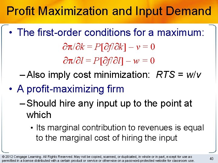
Profit Maximization and Input Demand • The first-order conditions for a maximum: / k = P[ f/ k] – v = 0 / l = P[ f/ l] – w = 0 – Also imply cost minimization: RTS = w/v • A profit-maximizing firm – Should hire any input up to the point at which • Its marginal contribution to revenues is equal to the marginal cost of hiring the input © 2012 Cengage Learning. All Rights Reserved. May not be copied, scanned, or duplicated, in whole or in part, except for use as permitted in a license distributed with a certain product or service or otherwise on a password-protected website for classroom use. 40

Profit Maximization and Input Demand • Marginal revenue product – The extra revenue a firm receives – When it uses one more unit of an input – In the price-taking case, MRPl = Pfl and MRPk = Pfk © 2012 Cengage Learning. All Rights Reserved. May not be copied, scanned, or duplicated, in whole or in part, except for use as permitted in a license distributed with a certain product or service or otherwise on a password-protected website for classroom use. 41

Profit Maximization and Input Demand • Second-order conditions: kk = fkk < 0 ll = fll < 0 kk ll - kl 2 = fkkfll – fkl 2 > 0 – Capital and labor must exhibit sufficiently diminishing marginal productivities so that marginal costs rise as output expands © 2012 Cengage Learning. All Rights Reserved. May not be copied, scanned, or duplicated, in whole or in part, except for use as permitted in a license distributed with a certain product or service or otherwise on a password-protected website for classroom use. 42

Input Demand Functions • Input demand functions Capital Demand = k(P, v, w) Labor Demand = l(P, v, w) – Are unconditional – They implicitly allow the firm to adjust its output to changing prices © 2012 Cengage Learning. All Rights Reserved. May not be copied, scanned, or duplicated, in whole or in part, except for use as permitted in a license distributed with a certain product or service or otherwise on a password-protected website for classroom use. 43

Single-Input Case • We expect l/ w 0 – Diminishing marginal productivity of labor • The first order condition for profit maximization was: Pft-w = F(l, w, p)= 0 – Finding the derivative of an implicit function © 2012 Cengage Learning. All Rights Reserved. May not be copied, scanned, or duplicated, in whole or in part, except for use as permitted in a license distributed with a certain product or service or otherwise on a password-protected website for classroom use. 44

Two-Input Case • For the case of two (or more inputs), the story is more complex – If there is a decrease in w, there will not only be a change in l but also a change in k as a new cost-minimizing combination of inputs is chosen • When k changes, the entire fl function changes • But, even in this case, l/ w 0 © 2012 Cengage Learning. All Rights Reserved. May not be copied, scanned, or duplicated, in whole or in part, except for use as permitted in a license distributed with a certain product or service or otherwise on a password-protected website for classroom use. 45

Two-Input Case • When w falls – Substitution effect • If output is held constant, there will be a tendency for the firm to want to substitute l for k in the production process – Output effect • A change in w will shift the firm’s expansion path • The firm’s cost curves will shift and a different output level will be chosen © 2012 Cengage Learning. All Rights Reserved. May not be copied, scanned, or duplicated, in whole or in part, except for use as permitted in a license distributed with a certain product or service or otherwise on a password-protected website for classroom use. 46

11. 5 The Substitution and Output Effects of a Decrease in the Price of a Factor (a) The isoquant map k period k 1 k 2 A (b) The output decision MC MC’ P C B Price q 2 q 1 l 2 l period q 1 q 2 Quantity period When the price of labor falls, two analytically different effects come into play. One of these, the substitution effect, would cause more labor to be purchased if output were held constant. This is shown as a movement from point A to point B in (a). At point B, the cost-minimizing condition (RTS = w/v) is satisfied for the new, lower w. This change in w/v will also shift the firm’s expansion path and its marginal cost curve. A normal situation might be for the MC curve to shift downward in response to a decrease in w as shown in (b). With this new curve ( MC’) a higher level of output (q 2) will be chosen. Consequently, the hiring of labor will increase (to l 2), also from this output effect. © 2012 Cengage Learning. All Rights Reserved. May not be copied, scanned, or duplicated, in whole or in part, except for use as permitted in a license distributed with a certain product or service or otherwise on a password-protected website for classroom use. 47

Cross-Price Effects • How capital usage responds to a wage change – No definite statement can be made – A fall in the wage will lead the firm to substitute away from capital – The output effect will cause more capital to be demanded as the firm expands production © 2012 Cengage Learning. All Rights Reserved. May not be copied, scanned, or duplicated, in whole or in part, except for use as permitted in a license distributed with a certain product or service or otherwise on a password-protected website for classroom use. 48

Substitution and Output Effects • When the price of an input falls – Two effects cause the quantity demanded of that input to rise: 1. The substitution effect causes any given output level to be produced using more of the input 2. The fall in costs causes more of the good to be sold, thereby creating an additional output effect that increases demand for the input © 2012 Cengage Learning. All Rights Reserved. May not be copied, scanned, or duplicated, in whole or in part, except for use as permitted in a license distributed with a certain product or service or otherwise on a password-protected website for classroom use. 49

Substitution and Output Effects • Two concepts of demand for any input – Conditional demand for labor, lc(v, w, q) – Unconditional demand for labor, l(P, v, w) – At the profit-maximizing level of output l(P, v, w) = lc(v, w, q(P, v, w)) © 2012 Cengage Learning. All Rights Reserved. May not be copied, scanned, or duplicated, in whole or in part, except for use as permitted in a license distributed with a certain product or service or otherwise on a password-protected website for classroom use. 50

Substitution and Output Effects • Differentiation with respect to w yields substitution effect output effect total effect © 2012 Cengage Learning. All Rights Reserved. May not be copied, scanned, or duplicated, in whole or in part, except for use as permitted in a license distributed with a certain product or service or otherwise on a password-protected website for classroom use. 51

11. 5 Decomposing Input Demand into Substitution and Output Components • Cobb–Douglas function • When one of the inputs is held fixed q = f(k, l, g) = k 0. 25 l 0. 25 g 0. 5 • Features: 1. Permits capital–labor substitution 2. Exhibits increasing marginal costs • Where • k is capital input • l is labor input • g is the size of the factory, held constant at 16 © 2012 Cengage Learning. All Rights Reserved. May not be copied, scanned, or duplicated, in whole or in part, except for use as permitted in a license distributed with a certain product or service or otherwise on a password-protected website for classroom use. 52

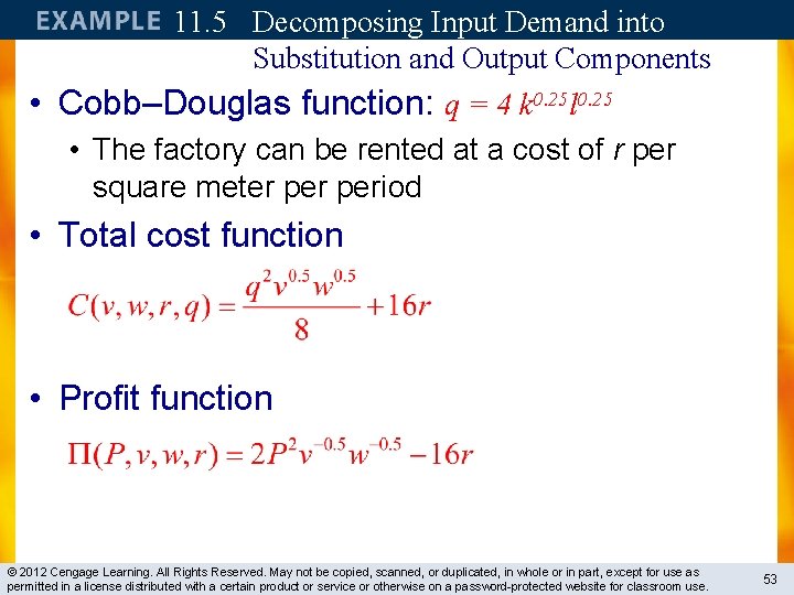
11. 5 Decomposing Input Demand into Substitution and Output Components • Cobb–Douglas function: q = 4 k 0. 25 l 0. 25 • The factory can be rented at a cost of r per square meter period • Total cost function • Profit function © 2012 Cengage Learning. All Rights Reserved. May not be copied, scanned, or duplicated, in whole or in part, except for use as permitted in a license distributed with a certain product or service or otherwise on a password-protected website for classroom use. 53

11. 5 Decomposing Input Demand into Substitution and Output Components • Envelope results • A change in the wage has a larger effect on total labor demand • Than it does on contingent labor demand • Because the exponent of w is more negative in the total demand equation © 2012 Cengage Learning. All Rights Reserved. May not be copied, scanned, or duplicated, in whole or in part, except for use as permitted in a license distributed with a certain product or service or otherwise on a password-protected website for classroom use. 54

Boundaries of the firm • Common features of alternative theories – Property rights theory – Transactions cost theory – Factors: uncertainty, complexity, and specialization © 2012 Cengage Learning. All Rights Reserved. May not be copied, scanned, or duplicated, in whole or in part, except for use as permitted in a license distributed with a certain product or service or otherwise on a password-protected website for classroom use. 55

Property rights theory • S(x. F, x. G) – Total surplus generated by the transaction between Fisher Body and GM • Bargaining: each firm receives half of the surplus – The sum of both firm’s profits • x. F – Investments made by Fisher Body • x. G – Investments made by GM © 2012 Cengage Learning. All Rights Reserved. May not be copied, scanned, or duplicated, in whole or in part, except for use as permitted in a license distributed with a certain product or service or otherwise on a password-protected website for classroom use. 56

Property rights theory • Efficient investment levels – Maximize total surplus minus investment costs S(x. F, x. G) - x. F - x. G • First-order conditions © 2012 Cengage Learning. All Rights Reserved. May not be copied, scanned, or duplicated, in whole or in part, except for use as permitted in a license distributed with a certain product or service or otherwise on a password-protected website for classroom use. 57

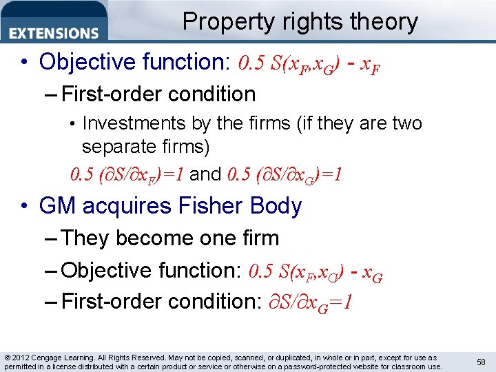
Property rights theory • Objective function: 0. 5 S(x. F, x. G) - x. F – First-order condition • Investments by the firms (if they are two separate firms) 0. 5 (∂S/∂x. F)=1 and 0. 5 (∂S/∂x. G)=1 • GM acquires Fisher Body – They become one firm – Objective function: 0. 5 S(x. F, x. G) - x. G – First-order condition: ∂S/∂x. G=1 © 2012 Cengage Learning. All Rights Reserved. May not be copied, scanned, or duplicated, in whole or in part, except for use as permitted in a license distributed with a certain product or service or otherwise on a password-protected website for classroom use. 58

Transactions cost theory • h. F – Costly action undertaken by Fisher Body at the time of bargaining - increases its bargaining power at the expense of GM – Haggling • h. G – Costly action undertaken by GM at the time of bargaining - increases its bargaining power at the expense of Fisher Body – Haggling © 2012 Cengage Learning. All Rights Reserved. May not be copied, scanned, or duplicated, in whole or in part, except for use as permitted in a license distributed with a certain product or service or otherwise on a password-protected website for classroom use. 59

Transactions cost theory • Bargaining shares – (h. F, h. G) - share accruing to Fisher Body – 1 - (h. F, h. G) - share accruing to GM – Where 0 < < 1, increasing in h. F and decreasing in h. G • Efficient levels of investment: x. F* and x. G* © 2012 Cengage Learning. All Rights Reserved. May not be copied, scanned, or duplicated, in whole or in part, except for use as permitted in a license distributed with a certain product or service or otherwise on a password-protected website for classroom use. 60

Transactions cost theory • Fisher Body’s objective function – Determining its equilibrium level of haggling (h. F, h. G) [S(x. F*, x. G*)- x. F* - x. G*]-h. F • First-order conditions © 2012 Cengage Learning. All Rights Reserved. May not be copied, scanned, or duplicated, in whole or in part, except for use as permitted in a license distributed with a certain product or service or otherwise on a password-protected website for classroom use. 61