Profit Maximization and Short Run Equilibrium In Perfect

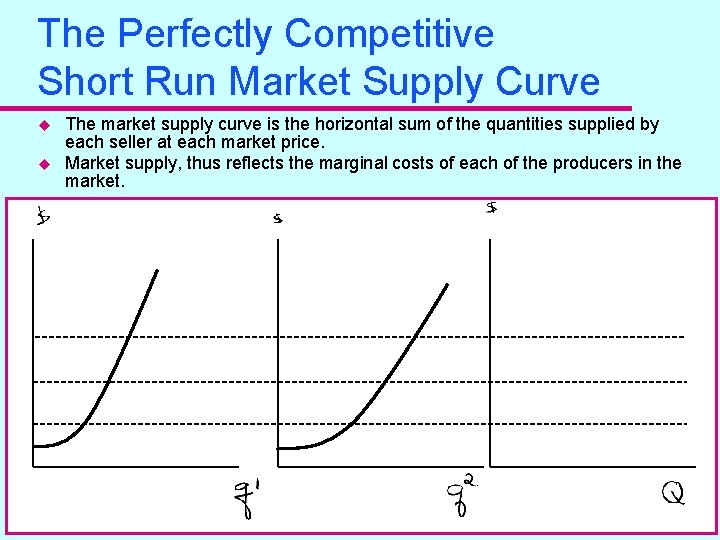
The Perfectly Competitive Short Run Market Supply Curve u u The market supply curve is the horizontal sum of the quantities supplied by each seller at each market price. Market supply, thus reflects the marginal costs of each of the producers in the market.

Reprise: The Short Run Market Supply u u How does our scratch supply curve compare to the one we bought off the shelf? Recall the supply function for X = mini speakers: QS = g(PX, Pfop, Poc, S&T, N) Where: QS = maximum quantity that producers are willing and able to sell PX = X’s price Pfop = the price of factors of production Poc = the opportunity costs S&T = science and technology N = number of firms in the market

Reprise: Producer’s Surplus – Again, Still u Recall that producer’s surplus measures the gain to the firm from selling all units at the market price. – PS on q units = Total Revenue – Variable Costs – PS on any particular unit = Price – Marginal Cost u We now know – Profit = Total Revenue – Variable Costs – Fixed Costs – Rearranging we get: » Variable Costs = Total Revenue – Fixed Costs – Profit – Plugging this expression for Variable Costs into PS we get: » PS on q units = Total Revenue – Total Revenue + Fixed Costs + Profit u So Producer’s Surplus can also be written as – PS on q units = Fixed Costs + Profit – An alternative interesting way to think of producer’s surplus u On the graph, Producer’s Surplus is – the area above the short run firm supply curve and below the market price

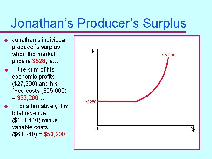
Jonathan’s Producer’s Surplus u u u Jonathan’s individual producer’s surplus when the market price is $528, is… …the sum of his economic profits ($27, 600) and his fixed costs ($25, 600) = $53, 200… … or alternatively it is total revenue ($121, 440) minus variable costs ($68, 240) = $53, 200. srs-firm ≈$250 0

SO: The Market & The Firm in Short Run Equilibrium u Given: – – u Market Demand Firms’ Technologies (including some fixed inputs) Factor Prices The Number of Firms Need: – Each firm is profit maximizing – Market Demand = Short Run Market Supply u Solve For: – – Q* q* P* profit*

SO: The Market & The Firm In Short Run Equilibrium $ $ Dmkt srmc A P* P* sratc a mr*=δ* atc @ q* SRSmkt w/N Q* MARKET Q If firms are identical then Q* = Nq* q* typical firm q

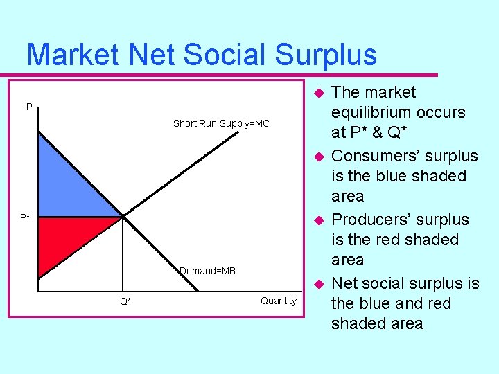
Market Net Social Surplus u P Short Run Supply=MC u P* u Demand=MB u Q* Quantity The market equilibrium occurs at P* & Q* Consumers’ surplus is the blue shaded area Producers’ surplus is the red shaded area Net social surplus is the blue and red shaded area

Next: Long Run Firm & Market Conduct u First, we are going to examine the long run cost curves of a single business. u Next, we will make precise the relation between the firm’s short run and long run supply decisions. u Then, we will consider the market in long run equilibrium. u So: Consider the following… – q = f(K, L) where q = firm’s output, K = capital, L = labor – PK = the unit price of capital & PL = unit price of labor – Both K and L are variable. » we are in the long run, since all inputs in the production function are variable!

(Mercifully Only) Three Long Run Cost Curves u There are three long run cost curves for the firm: – long run total cost (lrtc) lrtc = PLL*(q) + PKK*(q) – long run average total cost (lratc) lratc = lrtc/q – long run marginal cost (lrmc) lrmc = lrtc/ q u The one we will see/use most is the lratc curve.

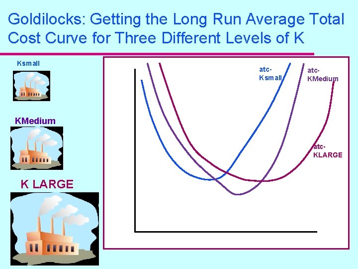
Goldilocks: Getting the Long Run Average Total Cost Curve for Three Different Levels of K Ksmall atc. KMedium atc. KLARGE K LARGE

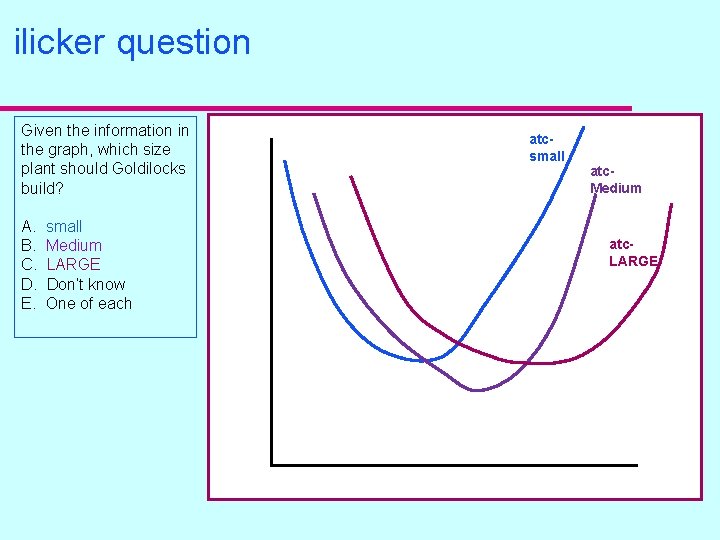
ilicker question Given the information in the graph, which size plant should Goldilocks build? A. B. C. D. E. small Medium LARGE Don’t know One of each atcsmall atc. Medium atc. LARGE

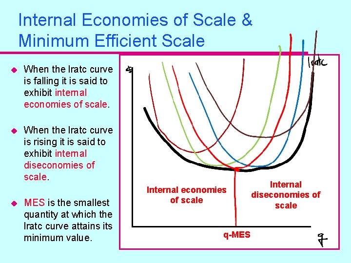
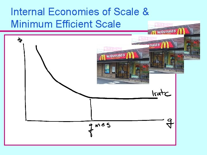
Internal Economies of Scale & Minimum Efficient Scale u When the lratc curve is falling it is said to exhibit internal economies of scale. u When the lratc curve is rising it is said to exhibit internal diseconomies of scale. u MES is the smallest quantity at which the lratc curve attains its minimum value. Internal economies of scale q-MES Internal diseconomies of scale

Ford, GM & Long Run Cost Curves

Internal Economies of Scale & Minimum Efficient Scale

Long Run ATC Curve in Relationship to Short Run ATC Curves u u When you are optimally designed, short run and long run cost values will coincide. As you deviate from what you planned for in the long run analysis, either producing more OR less than you optimally designed for, your short run costs will exceed your long run costs. $ sratc. Ksmall q=35 q=50 q=150 lratc q in tons

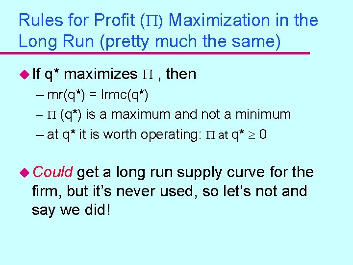
Rules for Profit ( ) Maximization in the Long Run (pretty much the same) u If q* maximizes , then – mr(q*) = lrmc(q*) – (q*) is a maximum and not a minimum – at q* it is worth operating: at q* 0 u Could get a long run supply curve for the firm, but it’s never used, so let’s not and say we did!

Long Run Equilibrium in Perfectly Competitive Markets u u u All the short run equilibrium properties hold. But also add… no firms wish to exit the market nor do firms want to enter. Given: market demand, factor prices and technology. . . Get: (P*, Q*, q*, N*) Note: For there to be neither entry or exit, need economic profit to be zero. This is a long run equilibrium requirement. Otherwise the number of firms in the market will still be in flux. – Short run profit invites entry. – Short run losses suggest exit. – If firms ARE NOT identical, then it’s really that the marginal firm has zero profit.

Why Are There Zero Economic Profits in the Long Run? u u u Zero economic profits means that all factors used in production make exactly their opportunity cost. Purchased factors receive their market price, which is equal to their opportunity cost. Owned factors receive the same compensation that they would receive in their next best use, which is also equal to their opportunity cost. Thus, no firm wants to enter the market because it cannot make any more money than it is currently making. Similarly, no firm wants to leave the market because it cannot make any more money in any other business.

Long Run Equilibrium Position with Identical Firms u Each firm is profit maximizing mr = mc at q* for each firm. (1) u Zero profit required P* = lratc at q* for each firm. (2) u Perfectly competitive firm P* = mr at all values of q. (3) u Sub (3) into (1) P* = mc at q* for each firm. (4) u Using (2) and (4) mc = lratc at q* for each firm. u Therefore, q* is at the minimum of the typical firm’s lratc curve. So. . . q* is at MES. – P* must be the price consistent with the minimum value on the typical firm’s lratc curve. – N* and Q* get determined by position of market demand.

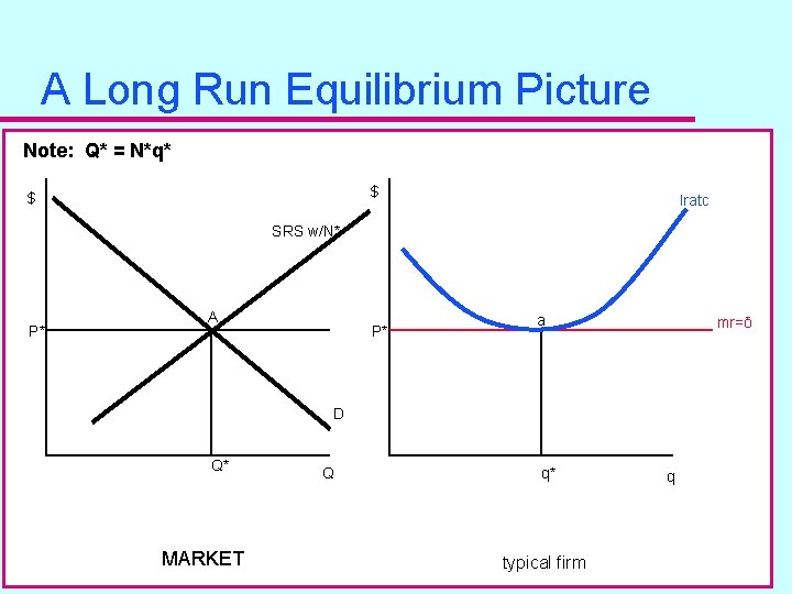
A Long Run Equilibrium Picture Note: Q* = N*q* $ $ lratc SRS w/N* P* A P* a mr=δ D Q* MARKET Q q* typical firm q

Steps to Draw the Picture? u Doesn’t matter how you draw it, as long as you draw it correctly in the end. u Draw-a-person tests.

What’s Not OK. . .