Production Power Point Slides prepared by Andreea CHIRITESCU

Production Power. Point Slides prepared by: Andreea CHIRITESCU, Eastern Illinois University; Modified by: Ronald WENDNER, University of Graz, Austria © 2012 Cengage Learning. All Rights Reserved. May not be copied, scanned, or duplicated, in whole or in part, except for use as permitted in a license distributed with a certain product or service or otherwise on a password-protected website for classroom use. 1

The Plan • Production and marginal/average productivity – Marginal rate of technical substitution – Elasticity of substitution • Returns to scale • Specific production functions – Linear – Fixed proportions – Cobb-Douglas; CES • Technical progress © 2012 Cengage Learning. All Rights Reserved. May not be copied, scanned, or duplicated, in whole or in part, except for use as permitted in a license distributed with a certain product or service or otherwise on a password-protected website for classroom use. 2

Production function • The firm’s production function – particular good (q) – maximum amount of q that can be produced – using alternative combinations of capital (k) and labor (l) q = f(k, l) - In more general settings: many inputs (and many outputs) production possibility sets Query. Identify important properties of a production function. © 2012 Cengage Learning. All Rights Reserved. May not be copied, scanned, or duplicated, in whole or in part, except for use as permitted in a license distributed with a certain product or service or otherwise on a password-protected website for classroom use. 3

Relations between output & inputs • Marginal product (MP) – additional output from 1 more unit of an input • Average product (AP) – output per unit of input © 2012 Cengage Learning. All Rights Reserved. May not be copied, scanned, or duplicated, in whole or in part, except for use as permitted in a license distributed with a certain product or service or otherwise on a password-protected website for classroom use. 4

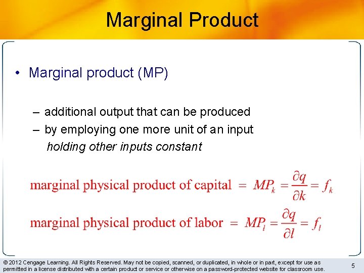
Marginal Product • Marginal product (MP) – additional output that can be produced – by employing one more unit of an input holding other inputs constant © 2012 Cengage Learning. All Rights Reserved. May not be copied, scanned, or duplicated, in whole or in part, except for use as permitted in a license distributed with a certain product or service or otherwise on a password-protected website for classroom use. 5

Diminishing Marginal Productivity • Marginal physical product – Depends on how much of that input is used • Diminishing marginal productivity © 2012 Cengage Learning. All Rights Reserved. May not be copied, scanned, or duplicated, in whole or in part, except for use as permitted in a license distributed with a certain product or service or otherwise on a password-protected website for classroom use. 6

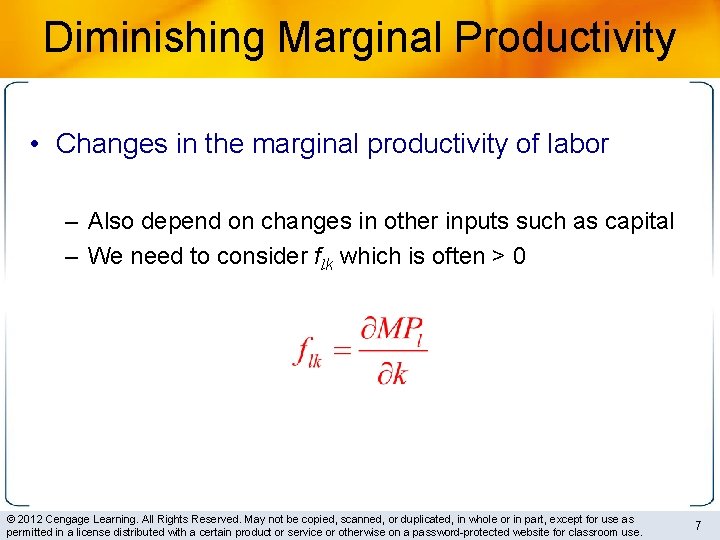
Diminishing Marginal Productivity • Changes in the marginal productivity of labor – Also depend on changes in other inputs such as capital – We need to consider flk which is often > 0 © 2012 Cengage Learning. All Rights Reserved. May not be copied, scanned, or duplicated, in whole or in part, except for use as permitted in a license distributed with a certain product or service or otherwise on a password-protected website for classroom use. 7

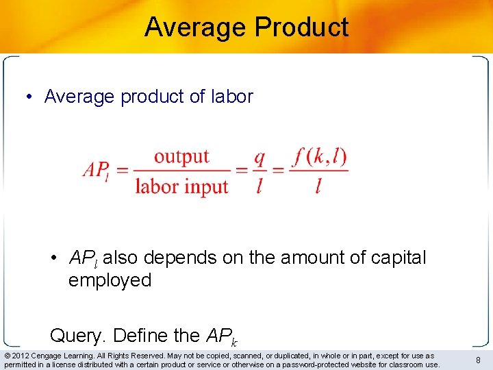
Average Product • Average product of labor • APl also depends on the amount of capital employed Query. Define the APk © 2012 Cengage Learning. All Rights Reserved. May not be copied, scanned, or duplicated, in whole or in part, except for use as permitted in a license distributed with a certain product or service or otherwise on a password-protected website for classroom use. 8

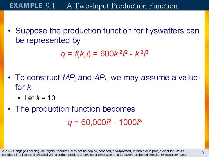
9. 1 A Two-Input Production Function • Suppose the production function for flyswatters can be represented by q = f(k, l) = 600 k 2 l 2 - k 3 l 3 • To construct MPl and APl, we may assume a value for k • Let k = 10 • The production function becomes q = 60, 000 l 2 - 1000 l 3 © 2012 Cengage Learning. All Rights Reserved. May not be copied, scanned, or duplicated, in whole or in part, except for use as permitted in a license distributed with a certain product or service or otherwise on a password-protected website for classroom use. 9

9. 1 A Two-Input Production Function • The marginal productivity function is MPl = ∂q/∂l = 120, 000 l - 3000 l 2 • Which diminishes as l increases • This implies that q has a maximum value: 120, 000 l - 3000 l 2 = 0 40 l = l 2 l = 40 • Labor input beyond l = 40 reduces output © 2012 Cengage Learning. All Rights Reserved. May not be copied, scanned, or duplicated, in whole or in part, except for use as permitted in a license distributed with a certain product or service or otherwise on a password-protected website for classroom use. 10

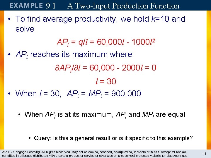
9. 1 A Two-Input Production Function • To find average productivity, we hold k=10 and solve APl = q/l = 60, 000 l - 1000 l 2 • APl reaches its maximum where ∂APl/∂l = 60, 000 - 2000 l = 0 l = 30 • When l = 30, APl = MPl = 900, 000 • When APl is at its maximum, APl and MPl are equal • Query: Is this a general result or is it specific to this example? © 2012 Cengage Learning. All Rights Reserved. May not be copied, scanned, or duplicated, in whole or in part, except for use as permitted in a license distributed with a certain product or service or otherwise on a password-protected website for classroom use. 11

Input substitution • So far: – how increase in one input raises output – how much output per unit of input • Next: Can inputs be substituted for each other? – graphically: isoquant maps – analytically: • marginal rate of technical substitution (MRTS or RTS) • elasticity of substitution © 2012 Cengage Learning. All Rights Reserved. May not be copied, scanned, or duplicated, in whole or in part, except for use as permitted in a license distributed with a certain product or service or otherwise on a password-protected website for classroom use. 12

Isoquant Maps • Isoquant map – illustrate the possible substitution of one input for another • An isoquant – those combinations of k and l that can produce a given(=fixed) level of output (q 0) f(k, l) = q 0 © 2012 Cengage Learning. All Rights Reserved. May not be copied, scanned, or duplicated, in whole or in part, except for use as permitted in a license distributed with a certain product or service or otherwise on a password-protected website for classroom use. 13

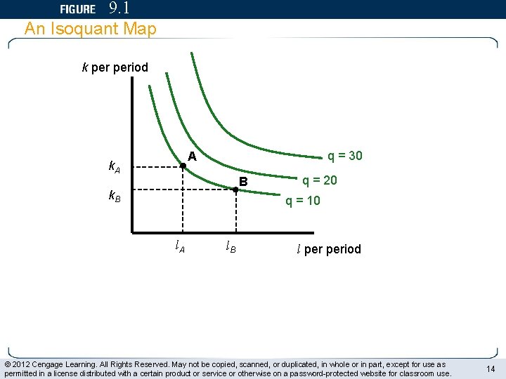
9. 1 An Isoquant Map k period q = 30 A k. A B k. B q = 20 q = 10 l. A l. B l period © 2012 Cengage Learning. All Rights Reserved. May not be copied, scanned, or duplicated, in whole or in part, except for use as permitted in a license distributed with a certain product or service or otherwise on a password-protected website for classroom use. 14

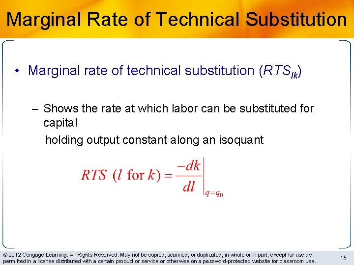
Marginal Rate of Technical Substitution • Marginal rate of technical substitution (RTSlk) – Shows the rate at which labor can be substituted for capital holding output constant along an isoquant © 2012 Cengage Learning. All Rights Reserved. May not be copied, scanned, or duplicated, in whole or in part, except for use as permitted in a license distributed with a certain product or service or otherwise on a password-protected website for classroom use. 15

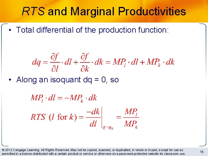
RTS and Marginal Productivities • Total differential of the production function: • Along an isoquant dq = 0, so © 2012 Cengage Learning. All Rights Reserved. May not be copied, scanned, or duplicated, in whole or in part, except for use as permitted in a license distributed with a certain product or service or otherwise on a password-protected website for classroom use. 16

RTS and Marginal Productivities • RTS will be positive (or zero) – Because MPl and MPk will both be nonnegative • Diminishing marginal productivity does not imply diminishing RTS • Diminishing RTS ☞ isoquants are convex – analytically: d(RTS)/dl < 0 © 2012 Cengage Learning. All Rights Reserved. May not be copied, scanned, or duplicated, in whole or in part, except for use as permitted in a license distributed with a certain product or service or otherwise on a password-protected website for classroom use. 17

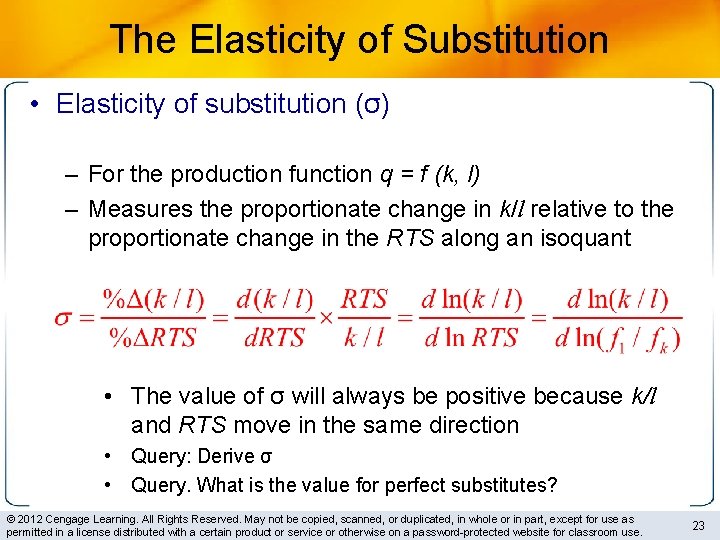
The Elasticity of Substitution • Elasticity of substitution (σ) – For the production function q = f (k, l) – Measures the proportionate change in k/l relative to the proportionate change in the RTS along an isoquant • The value of σ will always be positive because k/l and RTS move in the same direction • Query: Derive σ • Query. What is the value for perfect substitutes? © 2012 Cengage Learning. All Rights Reserved. May not be copied, scanned, or duplicated, in whole or in part, except for use as permitted in a license distributed with a certain product or service or otherwise on a password-protected website for classroom use. 23

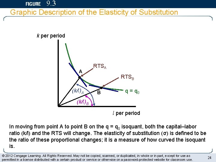
9. 3 Graphic Description of the Elasticity of Substitution k period A (k/l)A RTSB B q = q 0 (k/l)B l period In moving from point A to point B on the q = q 0 isoquant, both the capital–labor ratio (k/l) and the RTS will change. The elasticity of substitution (σ) is defined to be the ratio of these proportional changes; it is a measure of how curved the isoquant is. © 2012 Cengage Learning. All Rights Reserved. May not be copied, scanned, or duplicated, in whole or in part, except for use as permitted in a license distributed with a certain product or service or otherwise on a password-protected website for classroom use. 24

Elasticity of Substitution • If σ is high – The RTS will not change much relative to k/l – The isoquant will be relatively flat • If σ is low – The RTS will change by a substantial amount as k/l changes – The isoquant will be sharply curved • σ can change along an isoquant – Or as the scale of production changes © 2012 Cengage Learning. All Rights Reserved. May not be copied, scanned, or duplicated, in whole or in part, except for use as permitted in a license distributed with a certain product or service or otherwise on a password-protected website for classroom use. 25

What if inputs change simultaneously? • © 2012 Cengage Learning. All Rights Reserved. May not be copied, scanned, or duplicated, in whole or in part, except for use as permitted in a license distributed with a certain product or service or otherwise on a password-protected website for classroom use. 26

Returns to Scale • How does output respond to increases in all inputs together? – Suppose that all inputs are doubled, would output double? • As inputs are doubled. . . – Greater division of labor and specialization – higher efficiency – Loss in efficiency - management may become more difficult © 2012 Cengage Learning. All Rights Reserved. May not be copied, scanned, or duplicated, in whole or in part, except for use as permitted in a license distributed with a certain product or service or otherwise on a password-protected website for classroom use. 27

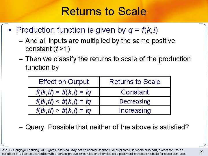
Returns to Scale • Production function is given by q = f(k, l) – And all inputs are multiplied by the same positive constant (t >1) – Then we classify the returns to scale of the production function by Effect on Output Returns to Scale f(tk, tl) = tf(k, l) = tq f(tk, tl) < tf(k, l) = tq f(tk, tl) > tf(k, l) = tq Constant Decreasing Increasing – Query. Possible that neither of the above is satisfied? © 2012 Cengage Learning. All Rights Reserved. May not be copied, scanned, or duplicated, in whole or in part, except for use as permitted in a license distributed with a certain product or service or otherwise on a password-protected website for classroom use. 28

Returns to Scale • Production function – Constant returns to scale for some levels of input usage – Increasing or decreasing returns for other levels – The degree of returns to scale is generally defined within a fairly narrow range of variation in input usage © 2012 Cengage Learning. All Rights Reserved. May not be copied, scanned, or duplicated, in whole or in part, except for use as permitted in a license distributed with a certain product or service or otherwise on a password-protected website for classroom use. 29

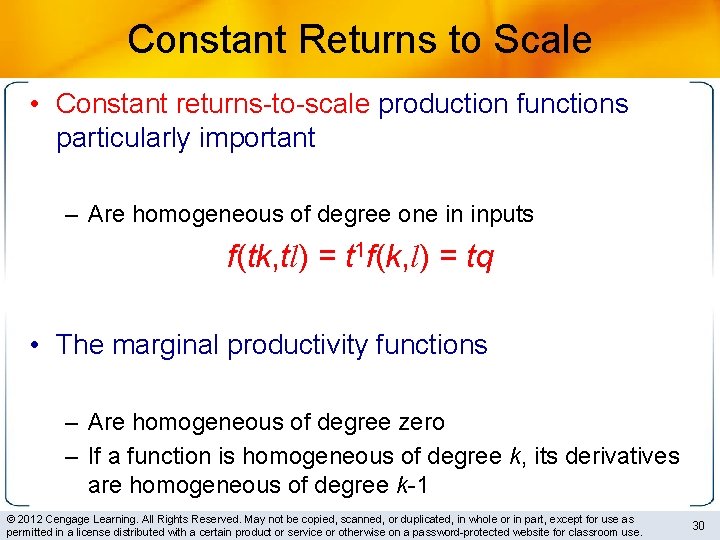
Constant Returns to Scale • Constant returns-to-scale production functions particularly important – Are homogeneous of degree one in inputs f(tk, tl) = t 1 f(k, l) = tq • The marginal productivity functions – Are homogeneous of degree zero – If a function is homogeneous of degree k, its derivatives are homogeneous of degree k-1 © 2012 Cengage Learning. All Rights Reserved. May not be copied, scanned, or duplicated, in whole or in part, except for use as permitted in a license distributed with a certain product or service or otherwise on a password-protected website for classroom use. 30

Constant Returns to Scale • Marginal productivity of any input – Depends on the ratio of capital and labor – Not on the absolute levels of these inputs • The MRTS between k and l – Depends only on the ratio of k to l – Not the scale of operation (q) – Holds for any homothetic production function • All of the isoquants are radial expansions of one another © 2012 Cengage Learning. All Rights Reserved. May not be copied, scanned, or duplicated, in whole or in part, except for use as permitted in a license distributed with a certain product or service or otherwise on a password-protected website for classroom use. 31

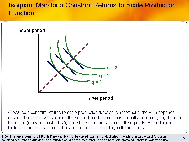
Isoquant Map for a Constant Returns-to-Scale Production Function k period q = 3 q = 2 q = 1 l period • Because a constant returns-to-scale production function is homothetic, the RTS depends only on the ratio of k to l, not on the scale of production. Consequently, along any ray through the origin (a ray of constant k/l), the RTS will be the same on all isoquants. An additional feature is that the isoquant labels increase proportionately with the inputs. © 2012 Cengage Learning. All Rights Reserved. May not be copied, scanned, or duplicated, in whole or in part, except for use as permitted in a license distributed with a certain product or service or otherwise on a password-protected website for classroom use. 32

Frequently Used Production Functions • Linear production function (σ = ∞) • Fixed-proportion production function (σ = 0) • Cobb-Douglas production function (σ = 1) • CES production function (σ >= 0) © 2012 Cengage Learning. All Rights Reserved. May not be copied, scanned, or duplicated, in whole or in part, except for use as permitted in a license distributed with a certain product or service or otherwise on a password-protected website for classroom use. 34

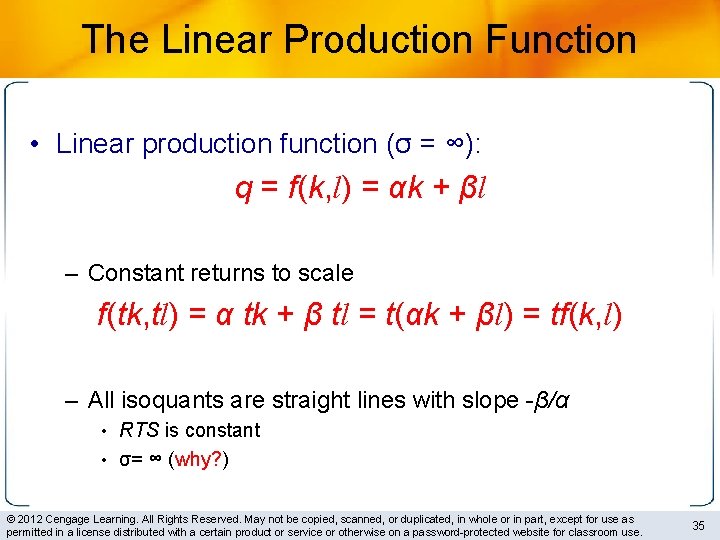
The Linear Production Function • Linear production function (σ = ∞): q = f(k, l) = αk + βl – Constant returns to scale f(tk, tl) = α tk + β tl = t(αk + βl) = tf(k, l) – All isoquants are straight lines with slope -β/α • RTS is constant • σ= ∞ (why? ) © 2012 Cengage Learning. All Rights Reserved. May not be copied, scanned, or duplicated, in whole or in part, except for use as permitted in a license distributed with a certain product or service or otherwise on a password-protected website for classroom use. 35

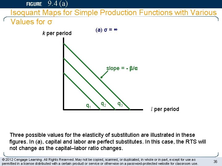
9. 4 (a) Isoquant Maps for Simple Production Functions with Various Values for σ (a) σ = ∞ k period slope = - β/α q 1 q 2 q 3 l period Three possible values for the elasticity of substitution are illustrated in these figures. In (a), capital and labor are perfect substitutes. In this case, the RTS will not change as the capital–labor ratio changes. © 2012 Cengage Learning. All Rights Reserved. May not be copied, scanned, or duplicated, in whole or in part, except for use as permitted in a license distributed with a certain product or service or otherwise on a password-protected website for classroom use. 36

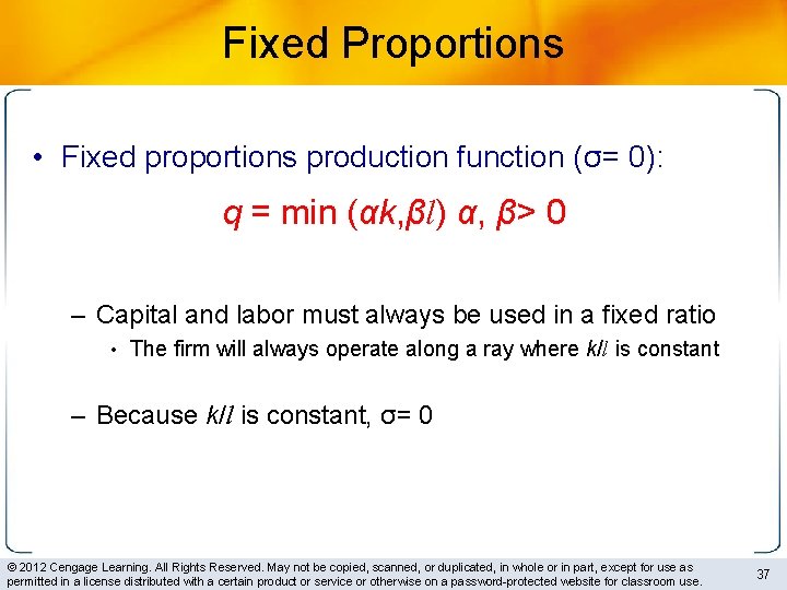
Fixed Proportions • Fixed proportions production function (σ= 0): q = min (αk, βl) α, β> 0 – Capital and labor must always be used in a fixed ratio • The firm will always operate along a ray where k/l is constant – Because k/l is constant, σ= 0 © 2012 Cengage Learning. All Rights Reserved. May not be copied, scanned, or duplicated, in whole or in part, except for use as permitted in a license distributed with a certain product or service or otherwise on a password-protected website for classroom use. 37

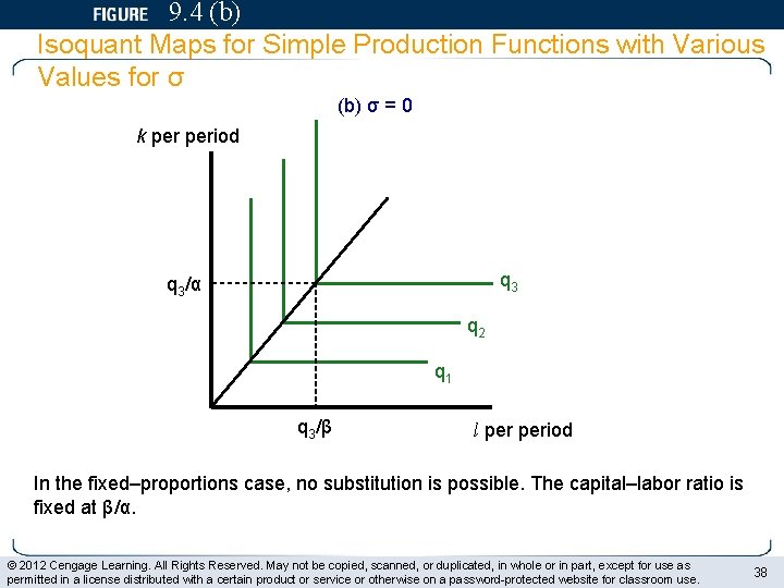
9. 4 (b) Isoquant Maps for Simple Production Functions with Various Values for σ (b) σ = 0 k period q 3/α q 2 q 1 q 3/β l period In the fixed–proportions case, no substitution is possible. The capital–labor ratio is fixed at β/α. © 2012 Cengage Learning. All Rights Reserved. May not be copied, scanned, or duplicated, in whole or in part, except for use as permitted in a license distributed with a certain product or service or otherwise on a password-protected website for classroom use. 38

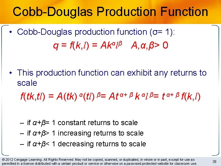
Cobb-Douglas Production Function • Cobb-Douglas production function (σ= 1): q = f(k, l) = Akαlβ A, α, β> 0 • This production function can exhibit any returns to scale f(tk, tl) = A(tk) α(tl) β= At α+ β k αl β= t α+ β f(k, l) – if α+β= 1 constant returns to scale – if α+β> 1 increasing returns to scale – if α+β< 1 decreasing returns to scale © 2012 Cengage Learning. All Rights Reserved. May not be copied, scanned, or duplicated, in whole or in part, except for use as permitted in a license distributed with a certain product or service or otherwise on a password-protected website for classroom use. 39

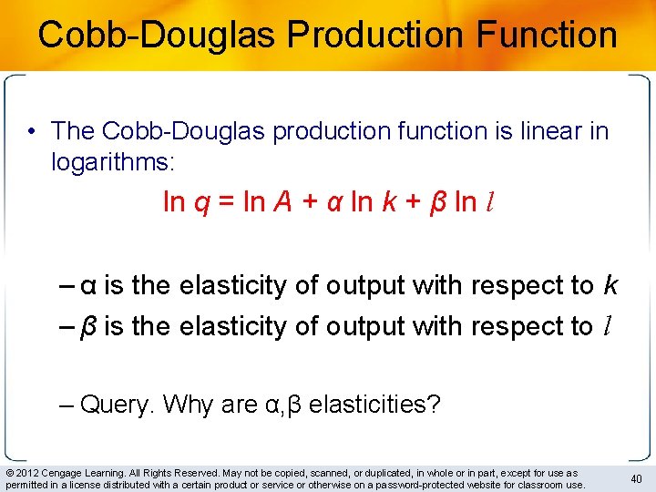
Cobb-Douglas Production Function • The Cobb-Douglas production function is linear in logarithms: ln q = ln A + α ln k + β ln l – α is the elasticity of output with respect to k – β is the elasticity of output with respect to l – Query. Why are α, β elasticities? © 2012 Cengage Learning. All Rights Reserved. May not be copied, scanned, or duplicated, in whole or in part, except for use as permitted in a license distributed with a certain product or service or otherwise on a password-protected website for classroom use. 40

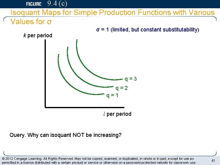
9. 4 (c) Isoquant Maps for Simple Production Functions with Various Values for σ k period σ = 1 (limited, but constant substitutability) q = 3 q = 2 q = 1 l period Query. Why can isoquant NOT be increasing? © 2012 Cengage Learning. All Rights Reserved. May not be copied, scanned, or duplicated, in whole or in part, except for use as permitted in a license distributed with a certain product or service or otherwise on a password-protected website for classroom use. 41

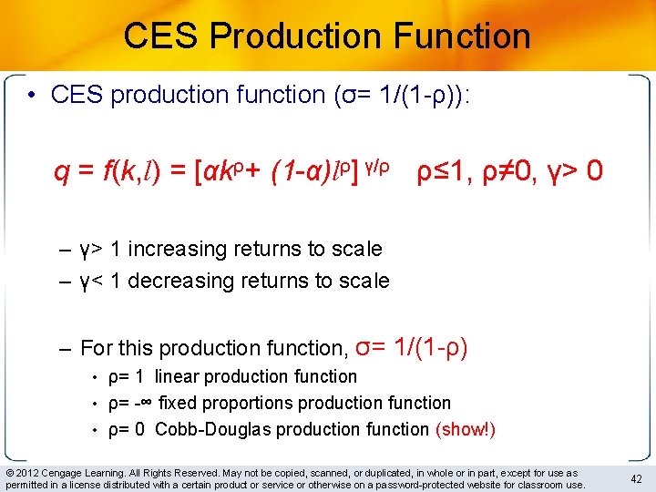
CES Production Function • CES production function (σ= 1/(1 -ρ)): q = f(k, l) = [αkρ+ (1 -α)lρ] γ/ρ ρ≤ 1, ρ≠ 0, γ> 0 – γ> 1 increasing returns to scale – γ< 1 decreasing returns to scale – For this production function, σ= 1/(1 -ρ) • ρ= 1 linear production function • ρ= -∞ fixed proportions production function • ρ= 0 Cobb-Douglas production function (show!) © 2012 Cengage Learning. All Rights Reserved. May not be copied, scanned, or duplicated, in whole or in part, except for use as permitted in a license distributed with a certain product or service or otherwise on a password-protected website for classroom use. 42

Technical Progress • Methods of production change over time – Following the development of superior production techniques • The same level of output can be produced with fewer inputs • The isoquant shifts towards origin © 2012 Cengage Learning. All Rights Reserved. May not be copied, scanned, or duplicated, in whole or in part, except for use as permitted in a license distributed with a certain product or service or otherwise on a password-protected website for classroom use. 43

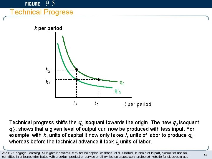
9. 5 Technical Progress k period k 2 k 1 q 0 q’ 0 l 1 l 2 l period Technical progress shifts the q 0 isoquant towards the origin. The new q 0 isoquant, q’ 0, shows that a given level of output can now be produced with less input. For example, with k 1 units of capital it now only takes l 1 units of labor to produce q 0, whereas before the technical advance it took l 2 units of labor. © 2012 Cengage Learning. All Rights Reserved. May not be copied, scanned, or duplicated, in whole or in part, except for use as permitted in a license distributed with a certain product or service or otherwise on a password-protected website for classroom use. 44

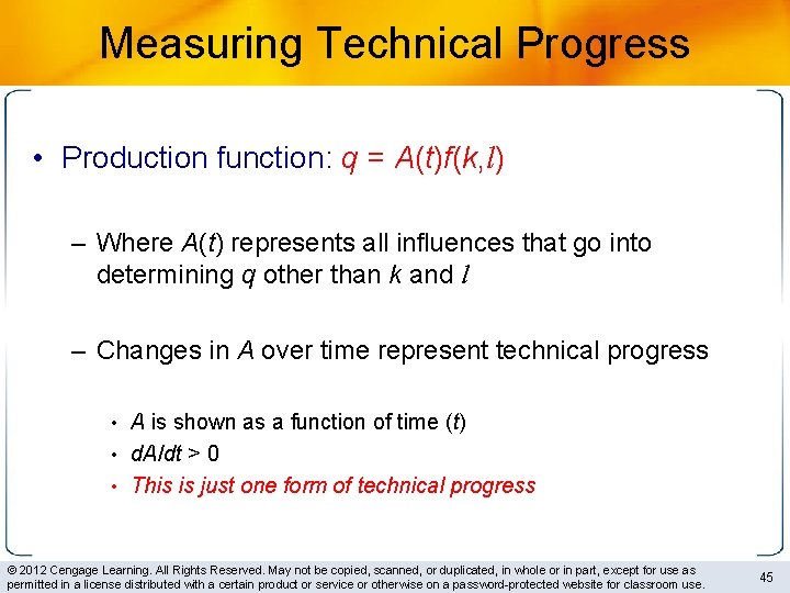
Measuring Technical Progress • Production function: q = A(t)f(k, l) – Where A(t) represents all influences that go into determining q other than k and l – Changes in A over time represent technical progress • A is shown as a function of time (t) • d. A/dt > 0 • This is just one form of technical progress © 2012 Cengage Learning. All Rights Reserved. May not be copied, scanned, or duplicated, in whole or in part, except for use as permitted in a license distributed with a certain product or service or otherwise on a password-protected website for classroom use. 45