Production Mix Problem lrg Graphical Solution 40 20

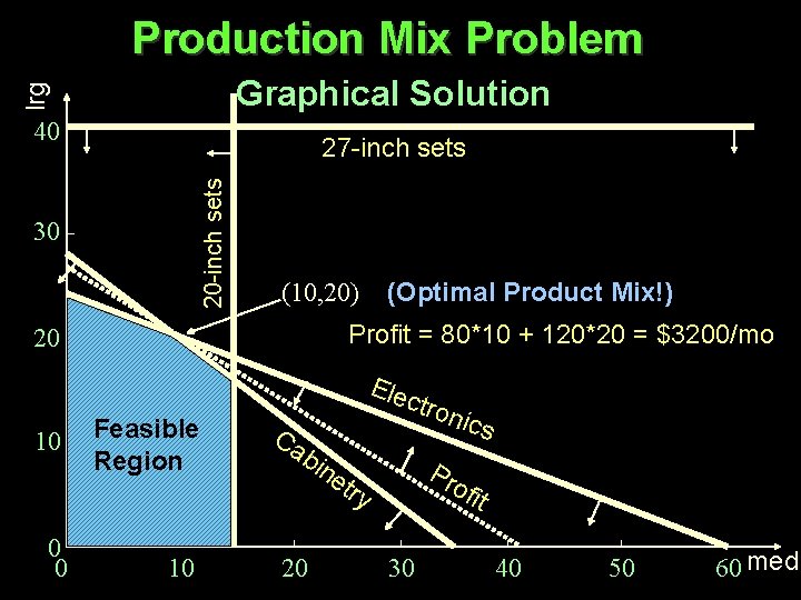
Production Mix Problem lrg Graphical Solution 40 20 -inch sets 27 -inch sets 30 (10, 20) (Optimal Product Mix!) Profit = 80*10 + 120*20 = $3200/mo 20 Ele 10 0 0 Feasible Region 10 Ca ctro bin Pr et ry 20 nics ofi 30 t 40 50 60 med

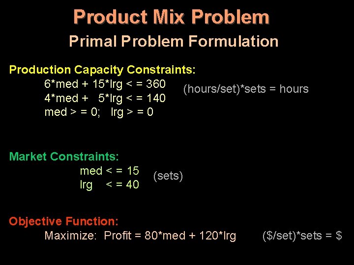
Product Mix Problem Primal Problem Formulation Production Capacity Constraints: 6*med + 15*lrg < = 360 (hours/set)*sets = hours 4*med + 5*lrg < = 140 med > = 0; lrg > = 0 Market Constraints: med < = 15 lrg < = 40 (sets) Objective Function: Maximize: Profit = 80*med + 120*lrg ($/set)*sets = $

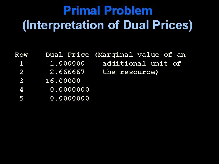
Primal Problem (Interpretation of Dual Prices) Row 1 2 3 4 5 Dual Price (Marginal value of an 1. 000000 additional unit of 2. 666667 the resource) 16. 00000 0. 0000000

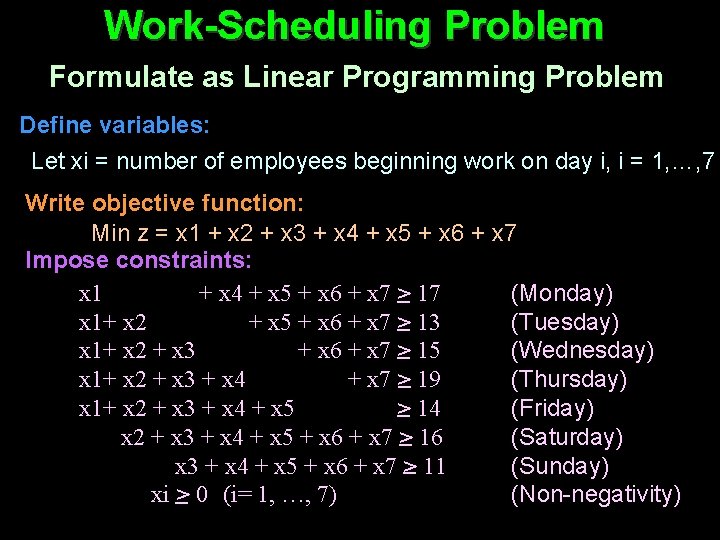
Work-Scheduling Problem Formulate as Linear Programming Problem Define variables: Let xi = number of employees beginning work on day i, i = 1, …, 7 Write objective function: Min z = x 1 + x 2 + x 3 + x 4 + x 5 + x 6 + x 7 Impose constraints: x 1 + x 4 + x 5 + x 6 + x 7 > 17 (Monday) x 1+ x 2 + x 5 + x 6 + x 7 > 13 (Tuesday) x 1+ x 2 + x 3 + x 6 + x 7 > 15 (Wednesday) x 1+ x 2 + x 3 + x 4 + x 7 > 19 (Thursday) x 1+ x 2 + x 3 + x 4 + x 5 > 14 (Friday) x 2 + x 3 + x 4 + x 5 + x 6 + x 7 > 16 (Saturday) x 3 + x 4 + x 5 + x 6 + x 7 > 11 (Sunday) xi > 0 (i= 1, …, 7) (Non-negativity)

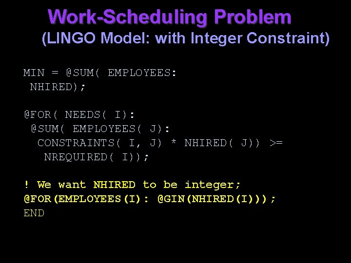
Work-Scheduling Problem (LINGO Model: with Integer Constraint) MIN = @SUM( EMPLOYEES: NHIRED); @FOR( NEEDS( I): @SUM( EMPLOYEES( J): CONSTRAINTS( I, J) * NHIRED( J)) >= NREQUIRED( I)); ! We want NHIRED to be integer; @FOR(EMPLOYEES(I): @GIN(NHIRED(I))); END

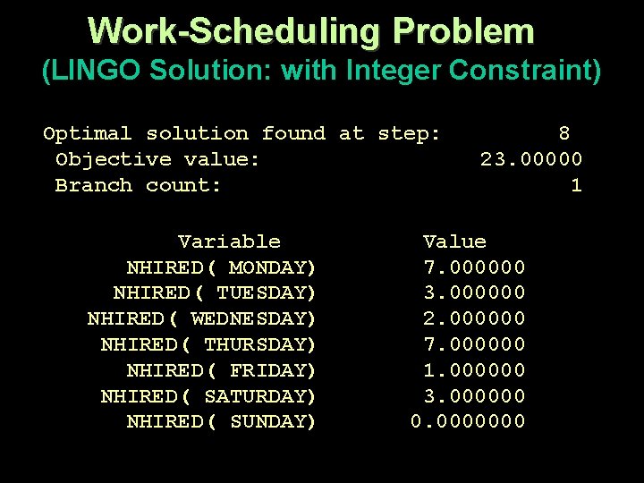
Work-Scheduling Problem (LINGO Solution: with Integer Constraint) Optimal solution found at step: Objective value: Branch count: Variable NHIRED( MONDAY) NHIRED( TUESDAY) NHIRED( WEDNESDAY) NHIRED( THURSDAY) NHIRED( FRIDAY) NHIRED( SATURDAY) NHIRED( SUNDAY) 8 23. 00000 1 Value 7. 000000 3. 000000 2. 000000 7. 000000 1. 000000 3. 000000 0. 0000000

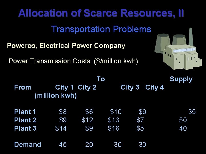
Allocation of Scarce Resources, II Transportation Problems Powerco, Electrical Power Company Power Transmission Costs: ($/million kwh) To From City 1 City 2 (million kwh) Plant 1 Plant 2 Plant 3 Demand Supply City 3 City 4 $8 $9 $14 $6 $12 $9 $10 $13 $16 $9 $7 $5 45 20 30 30 35 50 40

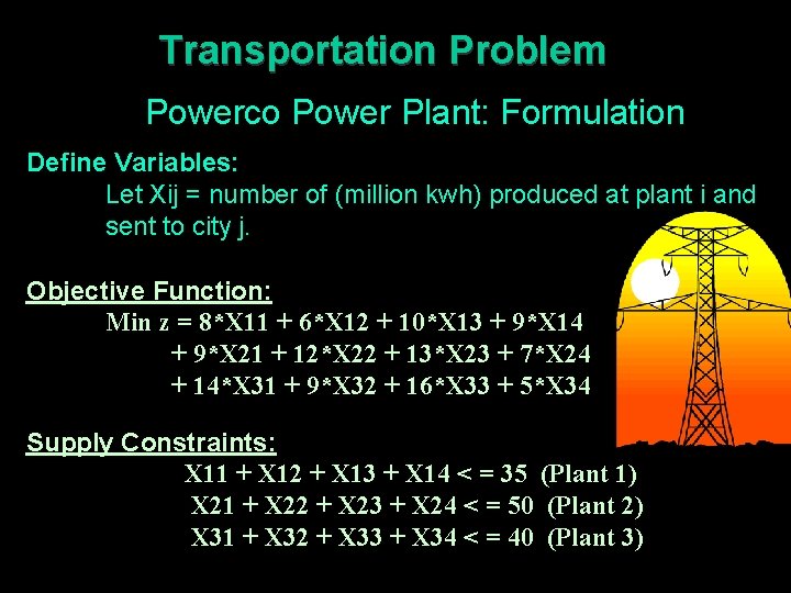
Transportation Problem Powerco Power Plant: Formulation Define Variables: Let Xij = number of (million kwh) produced at plant i and sent to city j. Objective Function: Min z = 8*X 11 + 6*X 12 + 10*X 13 + 9*X 14 + 9*X 21 + 12*X 22 + 13*X 23 + 7*X 24 + 14*X 31 + 9*X 32 + 16*X 33 + 5*X 34 Supply Constraints: X 11 + X 12 + X 13 + X 14 < = 35 (Plant 1) X 21 + X 22 + X 23 + X 24 < = 50 (Plant 2) X 31 + X 32 + X 33 + X 34 < = 40 (Plant 3)

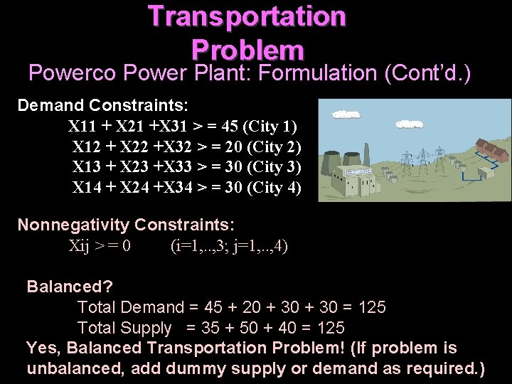
Transportation Problem Powerco Power Plant: Formulation (Cont’d. ) Demand Constraints: X 11 + X 21 +X 31 > = 45 (City 1) X 12 + X 22 +X 32 > = 20 (City 2) X 13 + X 23 +X 33 > = 30 (City 3) X 14 + X 24 +X 34 > = 30 (City 4) Nonnegativity Constraints: Xij > = 0 (i=1, . . , 3; j=1, . . , 4) Balanced? Total Demand = 45 + 20 + 30 = 125 Total Supply = 35 + 50 + 40 = 125 Yes, Balanced Transportation Problem! (If problem is unbalanced, add dummy supply or demand as required. )

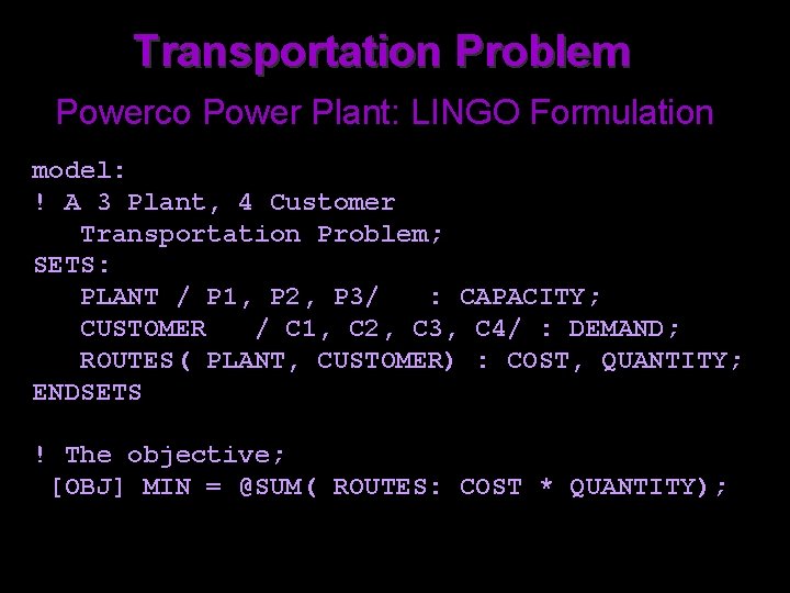
Transportation Problem Powerco Power Plant: LINGO Formulation model: ! A 3 Plant, 4 Customer Transportation Problem; SETS: PLANT / P 1, P 2, P 3/ : CAPACITY; CUSTOMER / C 1, C 2, C 3, C 4/ : DEMAND; ROUTES( PLANT, CUSTOMER) : COST, QUANTITY; ENDSETS ! The objective; [OBJ] MIN = @SUM( ROUTES: COST * QUANTITY);

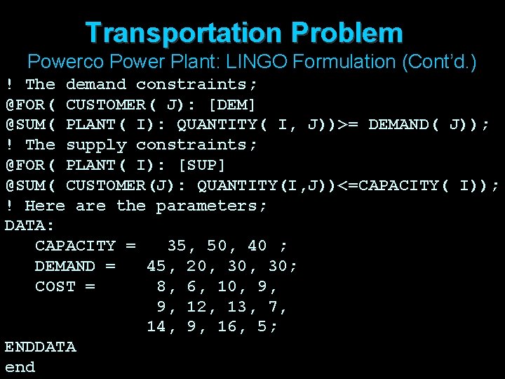
Transportation Problem Powerco Power Plant: LINGO Formulation (Cont’d. ) ! The demand constraints; @FOR( CUSTOMER( J): [DEM] @SUM( PLANT( I): QUANTITY( I, J))>= DEMAND( J)); ! The supply constraints; @FOR( PLANT( I): [SUP] @SUM( CUSTOMER(J): QUANTITY(I, J))<=CAPACITY( I)); ! Here are the parameters; DATA: CAPACITY = 35, 50, 40 ; DEMAND = 45, 20, 30; COST = 8, 6, 10, 9, 9, 12, 13, 7, 14, 9, 16, 5; ENDDATA end

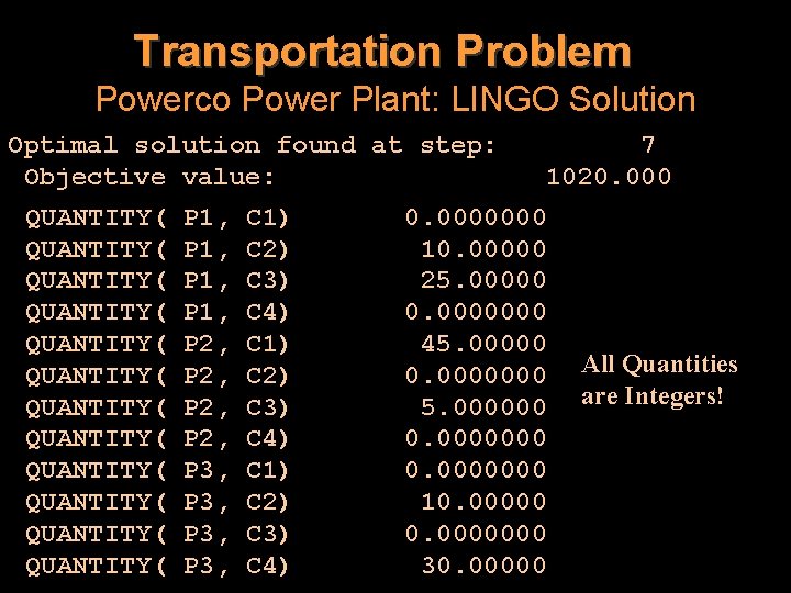
Transportation Problem Powerco Power Plant: LINGO Solution Optimal solution found at step: Objective value: QUANTITY( QUANTITY( QUANTITY( P 1, P 2, P 3, C 1) C 2) C 3) C 4) 7 1020. 0000000 10. 00000 25. 00000 0. 0000000 45. 00000 0. 0000000 5. 000000 0. 0000000 10. 0000000 30. 00000 All Quantities are Integers!

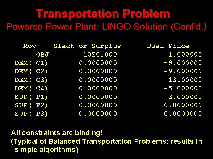
Transportation Problem Powerco Power Plant: LINGO Solution (Cont’d. ) Row Slack or Surplus OBJ 1020. 000 DEM( C 1) 0. 0000000 DEM( C 2) 0. 0000000 DEM( C 3) 0. 0000000 DEM( C 4) 0. 0000000 SUP( P 1) 0. 0000000 SUP( P 2) 0. 0000000 SUP( P 3) 0. 0000000 Dual Price 1. 000000 -9. 000000 -13. 00000 -5. 000000 3. 000000 0. 0000000 All constraints are binding! (Typical of Balanced Transportation Problems; results in simple algorithms)

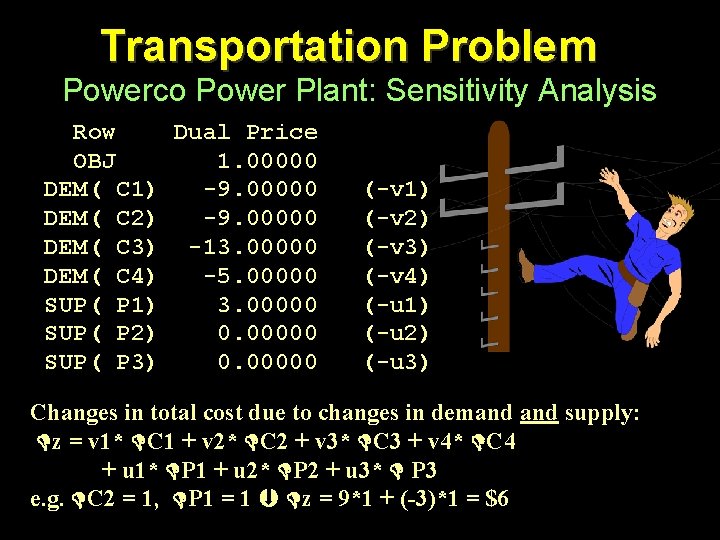
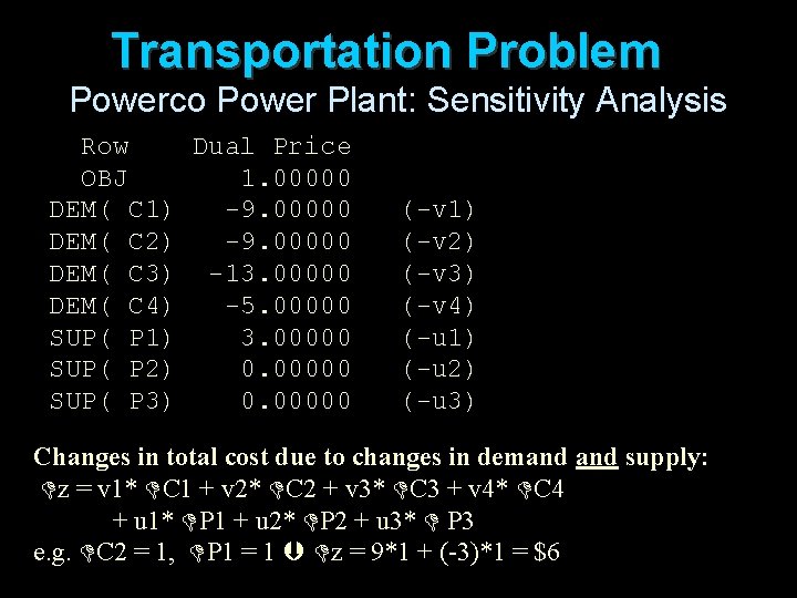
Transportation Problem Powerco Power Plant: Sensitivity Analysis Row Dual Price OBJ 1. 00000 DEM( C 1) -9. 00000 DEM( C 2) -9. 00000 DEM( C 3) -13. 00000 DEM( C 4) -5. 00000 SUP( P 1) 3. 00000 SUP( P 2) 0. 00000 SUP( P 3) 0. 00000 (-v 1) (-v 2) (-v 3) (-v 4) (-u 1) (-u 2) (-u 3) Changes in total cost due to changes in demand supply: z = v 1* C 1 + v 2* C 2 + v 3* C 3 + v 4* C 4 + u 1* P 1 + u 2* P 2 + u 3* P 3 e. g. C 2 = 1, P 1 = 1 z = 9*1 + (-3)*1 = $6

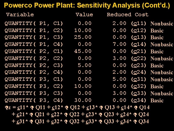
Powerco Power Plant: Sensitivity Analysis (Cont’d. ) Variable Value Reduced Cost QUANTITY( P 1, C 1) 0. 00 2. 00 (c 11) Nonbasic QUANTITY( P 1, C 2) 10. 00 (c 12) Basic QUANTITY( P 1, C 3) 25. 00 0. 00 (c 13) Basic QUANTITY( P 1, C 4) 0. 00 7. 00 (c 14) Nonbasic QUANTITY( P 2, C 1) 45. 00 0. 00 (c 21) Basic QUANTITY( P 2, C 2) 0. 00 3. 00 (c 22) Nonbasic QUANTITY( P 2, C 3) 5. 00 0. 00 (c 23) Basic QUANTITY( P 2, C 4) 0. 00 2. 00 (c 24) Nonbasic QUANTITY( P 3, C 1) 0. 00 5. 00 (c 31) Nonbasic QUANTITY( P 3, C 2) 10. 00 (c 32) Basic QUANTITY( P 3, C 3) 0. 00 3. 00 (c 33) Nonbasic QUANTITY( P 3, C 4) 30. 00 (c 34) Basic z = c 11* Q 11 + c 12* Q 12 + c 13* Q 13 + c 14* Q 14 + c 21* Q 21 + c 22* Q 22 + c 23* Q 23 + c 24* Q 24 + c 31* Q 31 + c 32* Q 32 + c 33* Q 33 + c 34* Q 34

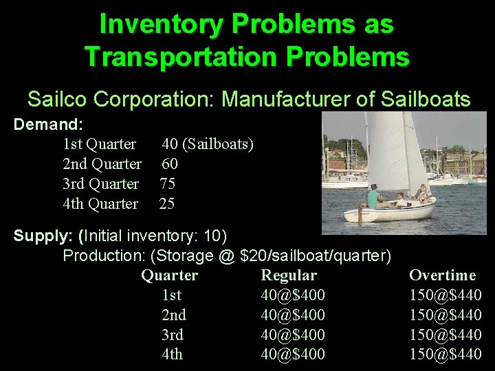
Inventory Problems as Transportation Problems Sailco Corporation: Manufacturer of Sailboats Demand: 1 st Quarter 2 nd Quarter 3 rd Quarter 4 th Quarter 40 (Sailboats) 60 75 25 Supply: (Initial inventory: 10) Production: (Storage @ $20/sailboat/quarter) Quarter Regular 1 st 40@$400 2 nd 40@$400 3 rd 40@$400 4 th 40@$400 Overtime 150@$440

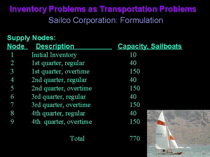
Inventory Problems as Transportation Problems Sailco Corporation: Formulation Supply Nodes: Node Description 1 Initial Inventory 2 1 st quarter, regular 3 1 st quarter, overtime 4 2 nd quarter, regular 5 2 nd quarter, overtime 6 3 rd quarter, regular 7 3 rd quarter, overtime 8 4 th quarter, regular 9 4 th quarter, overtime Total Capacity, Sailboats 10 40 150 770

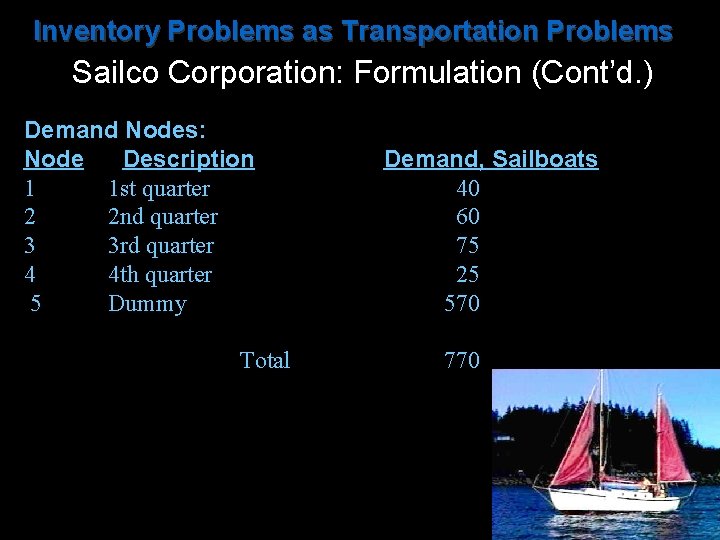
Inventory Problems as Transportation Problems Sailco Corporation: Formulation (Cont’d. ) Demand Nodes: Node Description 1 1 st quarter 2 2 nd quarter 3 3 rd quarter 4 4 th quarter 5 Dummy Total Demand, Sailboats 40 60 75 25 570 770

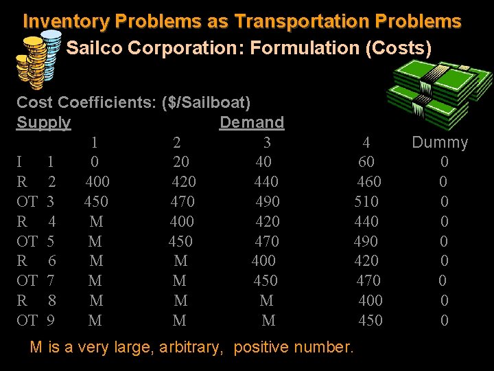
Inventory Problems as Transportation Problems Sailco Corporation: Formulation (Costs) Cost Coefficients: ($/Sailboat) Supply Demand 1 2 3 I 1 0 20 40 R 2 400 420 440 OT 3 450 470 490 R 4 M 400 420 OT 5 M 450 470 R 6 M M 400 OT 7 M M 450 R 8 M M M OT 9 M M M 4 60 460 510 440 490 420 470 400 450 M is a very large, arbitrary, positive number. Dummy 0 0 0 0 0

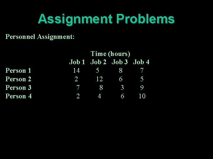
Assignment Problems Personnel Assignment: Person 1 Person 2 Person 3 Person 4 Time (hours) Job 1 Job 2 Job 3 Job 4 14 5 8 7 2 12 6 5 7 8 3 9 2 4 6 10

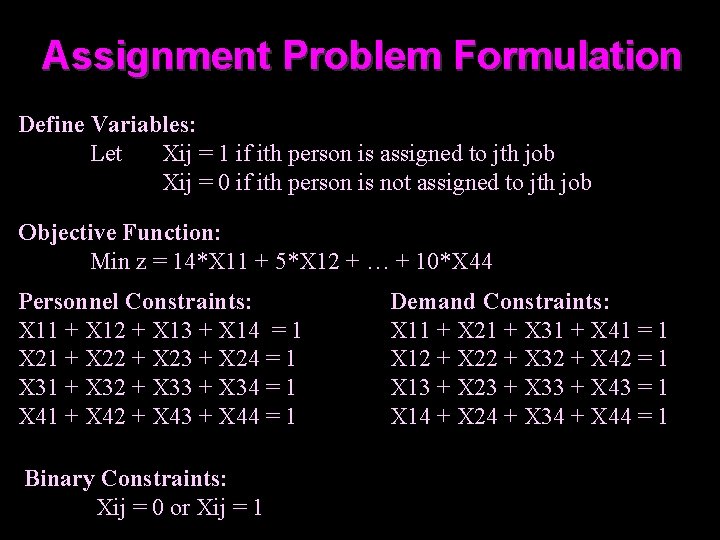
Assignment Problem Formulation Define Variables: Let Xij = 1 if ith person is assigned to jth job Xij = 0 if ith person is not assigned to jth job Objective Function: Min z = 14*X 11 + 5*X 12 + … + 10*X 44 Personnel Constraints: X 11 + X 12 + X 13 + X 14 = 1 X 21 + X 22 + X 23 + X 24 = 1 X 31 + X 32 + X 33 + X 34 = 1 X 41 + X 42 + X 43 + X 44 = 1 Binary Constraints: Xij = 0 or Xij = 1 Demand Constraints: X 11 + X 21 + X 31 + X 41 = 1 X 12 + X 22 + X 32 + X 42 = 1 X 13 + X 23 + X 33 + X 43 = 1 X 14 + X 24 + X 34 + X 44 = 1

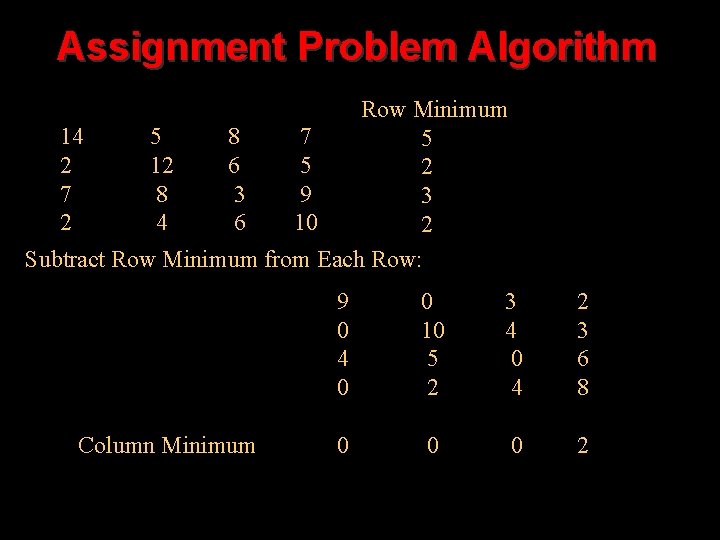
Assignment Problem Algorithm Row Minimum 14 5 8 7 5 2 12 6 5 2 7 8 3 9 3 2 4 6 10 2 Subtract Row Minimum from Each Row: Column Minimum 9 0 4 0 0 10 5 2 3 4 0 4 2 3 6 8 0 0 0 2

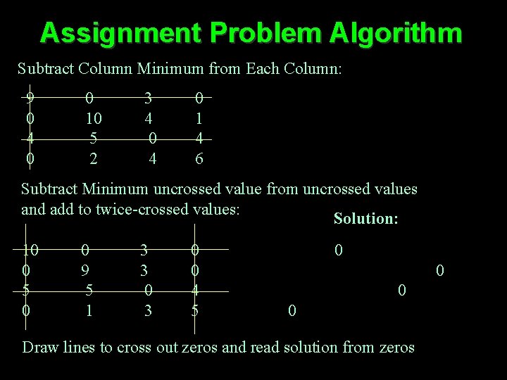
Assignment Problem Algorithm Subtract Column Minimum from Each Column: 9 0 4 0 0 10 5 2 3 4 0 1 4 6 Subtract Minimum uncrossed value from uncrossed values and add to twice-crossed values: Solution: 10 0 5 0 0 9 5 1 3 3 0 0 4 5 0 0 Draw lines to cross out zeros and read solution from zeros

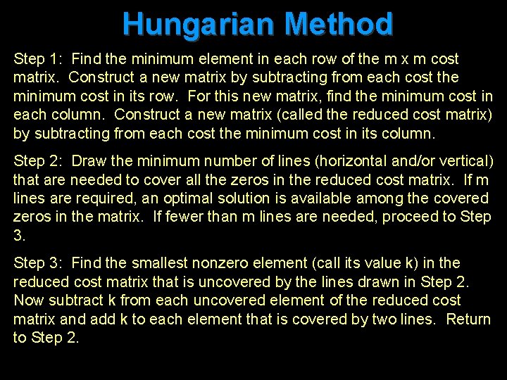
Hungarian Method Step 1: Find the minimum element in each row of the m x m cost matrix. Construct a new matrix by subtracting from each cost the minimum cost in its row. For this new matrix, find the minimum cost in each column. Construct a new matrix (called the reduced cost matrix) by subtracting from each cost the minimum cost in its column. Step 2: Draw the minimum number of lines (horizontal and/or vertical) that are needed to cover all the zeros in the reduced cost matrix. If m lines are required, an optimal solution is available among the covered zeros in the matrix. If fewer than m lines are needed, proceed to Step 3: Find the smallest nonzero element (call its value k) in the reduced cost matrix that is uncovered by the lines drawn in Step 2. Now subtract k from each uncovered element of the reduced cost matrix and add k to each element that is covered by two lines. Return to Step 2.