Production Function and Equilibrium in Labor Market Classical

Production Function and Equilibrium in Labor Market

Classical Model: Production Function • A central relationship in the classical model is the aggregate production function. • The production function, which is based on the technology of individual firms, is a relationship between the level of output and the level of factor inputs • Assume there are two inputs—Labor and capital. Due to the assumption of short-run, output will be a function of Labor (N) with capital constant (K), that is, output can be increased only by increasing the variable factor (N) with fixed factor (K) constant.

Y =F( , N) • Where K → Constant capital stock, N → Quantity of homogeneous Labor Input, Y → Real Output. • The short-run production function plotted below in Figure 2 -1 a is a technological relationship that determines the level of output given the level of labor input (employment). The capital stock, along with the existing level of technology and skill level of the workforce, is being held constant.

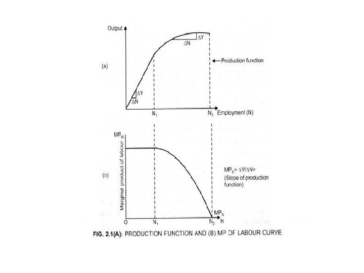
• As MPN represents addition to output when the Labor input is increased, MPN curve represents the slope of production function. MPN = ∆Y/∆N • The slope of the production function (MPN) is positive but decreases as we move along the curve. Characteristics of Production Function: • In short run, production function shows technological relationship between the output level (Y) and the level of employment (N). 1. At low level of Labor input before N 1 • The Production function is a straight line which exhibits constant returns to scale. • Therefore, MPN curve is flat which represents constant MPN. • It shows at very low level of output as we employ more labor to the given capital, productivity of the last worker added does not fall. • Therefore, MPN does not fall.

2. After N, till N 2 • As we add more labor, output increases but at a decreasing rate (i. e. , increment to the output decreases) MPN decreases but is positive. • This the area of diminishing returns to scale. In this area on the production function, total output increases at a diminishing rate due to the law of diminishing returns. • This law states that as variable inputs (in this case, homogeneous labor) are added to a fixed input (the capital stock, which is being held constant), beyond some point, the amount by which output increases will diminish.

3. Beyond N 2 • The additional Labor employed will not lead to additional production/ output i. e, MPN = 0. • Therefore, MPN curve touches X-axis at N 2. • At this point, both total output and marginal output decreased. Firms would not hire in the area of negative returns to scale.

Employment • Classical economists assumed that the quantity of labor employed would be determined by the forces of demand supply in the labor market. • The Amount of Labor employed will be determined at the point where: Aggregate Demand for Labor (Nd) = Aggregate Supply of Labor (Ns)

Assumptions 1. The market works well. Firms and individual workers optimize. 2. They have perfect information about relevant prices. 3. Money wage is adjusted automatically by the market. 4. Perfect competition.

Labor Demand • Demand for labor is negatively related to the real wages (W/P). This is because real wages are the cost of production for the firms. • Therefore, an increase in real wages due to increase in wages will lead to an increase in the cost of production. • This in turn will decrease the profits of the firm because profit is equal to Revenue minus cost (Profit = Revenue – Cost). • Due to decrease in the profit level, firm will demand less labor.

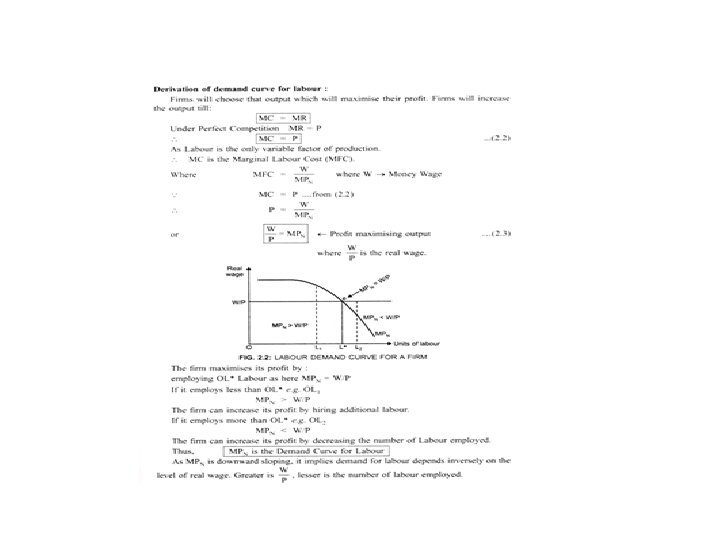
• Thus, the profit-maximizing quantity of labor demanded by a firm at each real wage is given by the labor input that equates the real wage and the MPN. • The marginal product curve is the firm’s demand curve for labor. • The implication is that labor demand depends inversely on the level of the real wage. The labor demand curve is downward sloping due to the law of diminishing returns. • The higher the real wage, for example, the lower the level of labor input that will equate the real wage to the MPN.

• The demand curve for labor is an economy wide aggregation of the individual firms’ demand curves. • For each real wage, this curve will give the sum of the quantities of labor input demanded by the firms in the economy. We write this aggregate labor Demand function (ND) as • ND = f (W/P) (-ve relation b/w ND and W/P ) …(1. 1)

Labor Supply • Supply of labor is positively related to the real wages (W/P). • This is because wages are the income of the laborer. Increase in wages implies increase in income, therefore, a labor is willing to work more at higher wages. • Thus, the supply curve of labor is positively sloped.

Derivation of Supply Curve of labor • Labor supply curve is derived from the income -leisure trade-off curve which shows the trade -off between leisure and work. • The figure 2. 3 below explain the individual labor supply decision

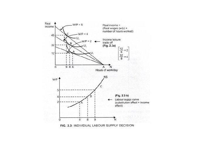
• At lower income level, labor prefers work to leisure → Substitution Effect (SE) > Income Effect (IE) • At ‘extremely’ higher income level, labor prefers leisure to work → IE > SE. Thus, we get backward bending supply curve of labor. • However ‘extremely’ high wages are rare. Therefore, it is assumed that the Aggregate labor supply curve has a positive slope. SE is strong enough to offset the IE. (SE > IE)

• Individual will supply labor up to the point where: • Slope of income leisure trade off line (shown by the slope of budget line) is equal to the slope of income leisure trade off curve (slope of Indifference Curve).

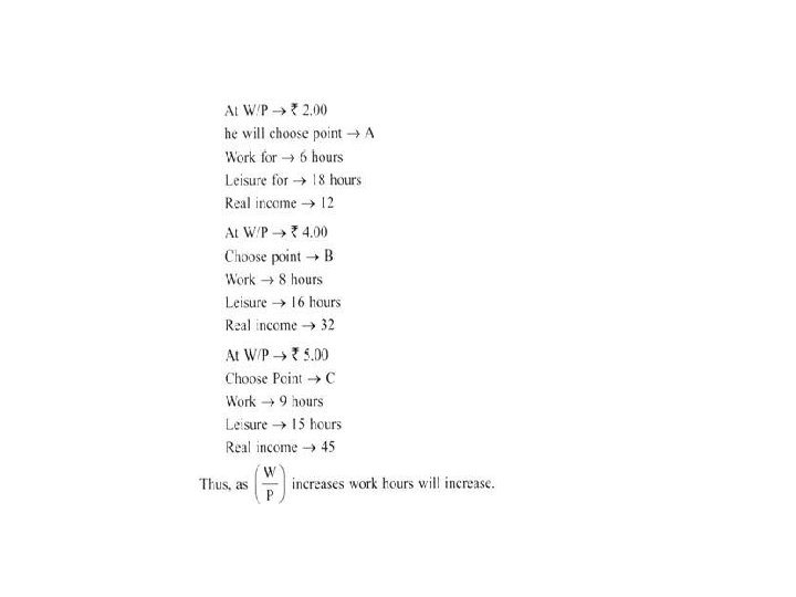
• In Fig. (2. 3 b), by plotting A, B, C at real wages 2. 00, 4. 00 and 5. 00, respectively, we get the labor supply curve which has a positive slope, showing as (W/P) increases more labor is willing to work.

Aggregate Supply Curve of Labor (Ns): • It is a horizontal summation of all individual labor supply curves. It gives the total labor supplied at each level of real wages. It is positively related to the real wages. • Ns = f (W/P) (+ve relation b/w Ns and W/P ) …(2. 5)

• In the labor market, the demand for labor and the supply of labor determine the level of output and employment. The classical economists regard the demand for labor as the function of the real wage rate: DN =f (W/P) • Where DN = demand for labor, W = wage rate and P = price level. Dividing wage rate (W) by price level (P), we get the real wage rate (W/P). • The demand for labor is a decreasing function of the real wage rate, as shown by the downward sloping DN curve in Fig. 2. It is by reducing the real wage rate that more workers can be employed.

Graph Labor Market Equilibrium

• The supply of labor also depends on the real wage rate: SN =f (W/P), where SN is the supply of labour. But it is an increasing function of the real wage rate, as shown by the upward sloping SN curve in Fig. 2. It is by increasing the real wage rate that more workers can be employed. • When the DN and SN curves intersect at point E, the full employment level NF is determined at the equilibrium real wage rate W/P 0. If the wage rate rises from WP 0 to WP 1 the supply of labor will be more than its demand by ds. • Now at W/P 1 wage rate, ds workers will be involuntary unemployed because the demand for labor (W/P 1 -d) is less than their supply (W/P 1 -s). With competition among workers for work, they will be willing to accept a lower wage rate. Consequently, the wage rate will fall from W/P 1 to W/P 0.

Equilibrium Output and Employment

• The supply of labor will fall and the demand for labor will rise and the equilibrium point E will be restored along with the full employment level Nr On the contrary, if the wage rate falls from W/P 0 to WP 2 the demand for labor (W/P 2 -d 1) will be more than its supply (W/P 2 -s 1). Competition by employers for workers will raise the wage rate from W/ P 2 to W/P 0 and the equilibrium point E will be restored along with the full employment level NF.

Graph related to Classical Output and Employment Determination

Explanation of Graph • Part above depicts labor market equilibrium at the real wage (W/P)* at equilibrium point A. In the aggregate, labor supply equals labor demand, Nd = Ns. • Equilibrium employment is N*. • Substitution of equilibrium employment into the production function in part b determines equilibrium aggregate output, Y* at point A. • Therefore, Equilibrium level of employment → N*, as here Nd = Ns shown by point ‘e’ • Real wage → (W/P)* (Fig. 2. 4 a) • Equilibrium level of output →Y* (Fig. 2. 4 b) • Thus, Y* is the full employment level.