Production Costs AP Microeconomics Unit 3 Days 1

Production & Costs AP Microeconomics Unit 3, Days 1 & 2 Stater

A few key terms: v. Firm: an organization that utilizes resources to produce a good or service that it hopes to sell profitably v. Explicit costs: direct, purchased, out-ofpocket costs. Examples? v. Implicit costs: indirect, non-purchased costs. • Includes the costs of the next-best alternatives that have been forgone… the opportunity costs!

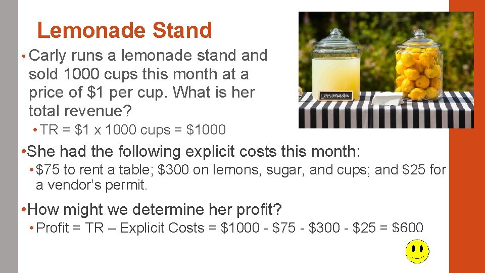
Lemonade Stand • Carly runs a lemonade stand sold 1000 cups this month at a price of $1 per cup. What is her total revenue? • TR = $1 x 1000 cups = $1000 • She had the following explicit costs this month: • $75 to rent a table; $300 on lemons, sugar, and cups; and $25 for a vendor’s permit. • How might we determine her profit? • Profit = TR – Explicit Costs = $1000 - $75 - $300 - $25 = $600

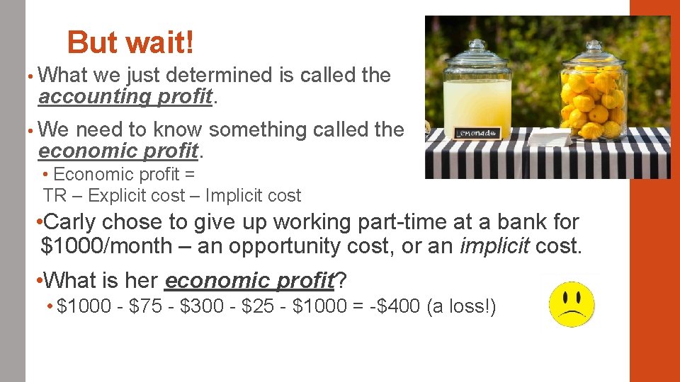
But wait! • What we just determined is called the accounting profit. • We need to know something called the economic profit. • Economic profit = TR – Explicit cost – Implicit cost • Carly chose to give up working part-time at a bank for $1000/month – an opportunity cost, or an implicit cost. • What is her economic profit? • $1000 - $75 - $300 - $25 - $1000 = -$400 (a loss!)

“Nothing is free; it is just nonpriced. ” • Economists always considers opportunity costs! We will use: • Economic costs: both explicit & implicit costs. • Economic profit: TR – explicit costs – implicit costs

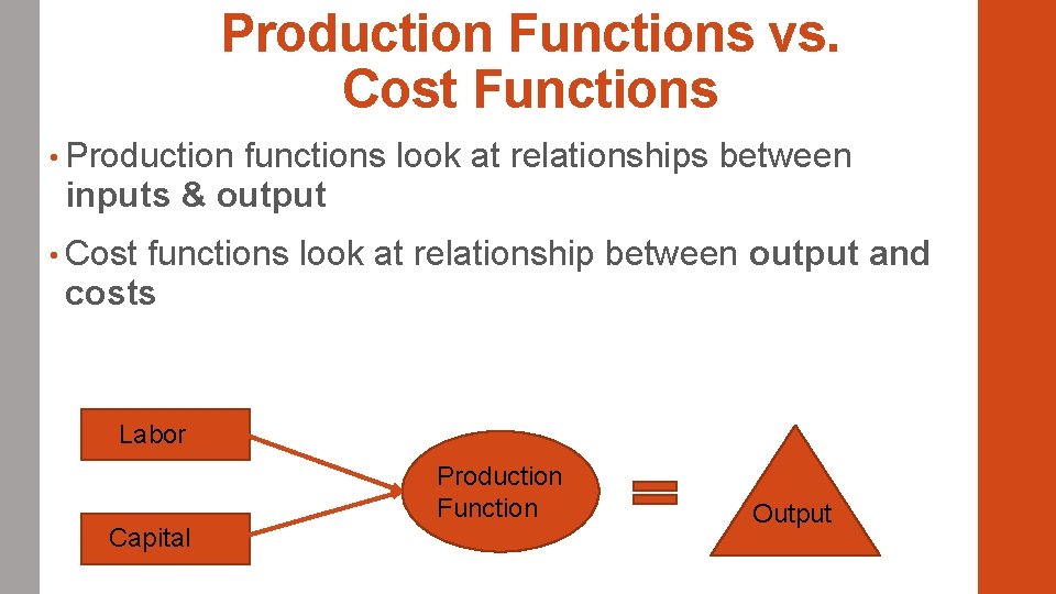
Production Functions vs. Cost Functions • Production functions look at relationships between inputs & output • Cost functions look at relationship between output and costs Labor Production Function Capital Output

Two Types of Inputs • Fixed inputs: resources that go into the production process that can’t be changed in the short run • Variable inputs: resources that can be adjusted in the short run to meet changes in demand • Ex: The firm can’t change the factory size in the short run, but it can add or reduce labor units (employees). • (also compare: fixed costs vs. variable costs)

Relationship between Productivity & Cost • High productivity implies low cost! • Inefficiency leads to high production costs – a competitive disadvantage

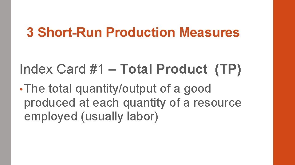
3 Short-Run Production Measures Index Card #1 – Total Product (TP) • The total quantity/output of a good produced at each quantity of a resource employed (usually labor)

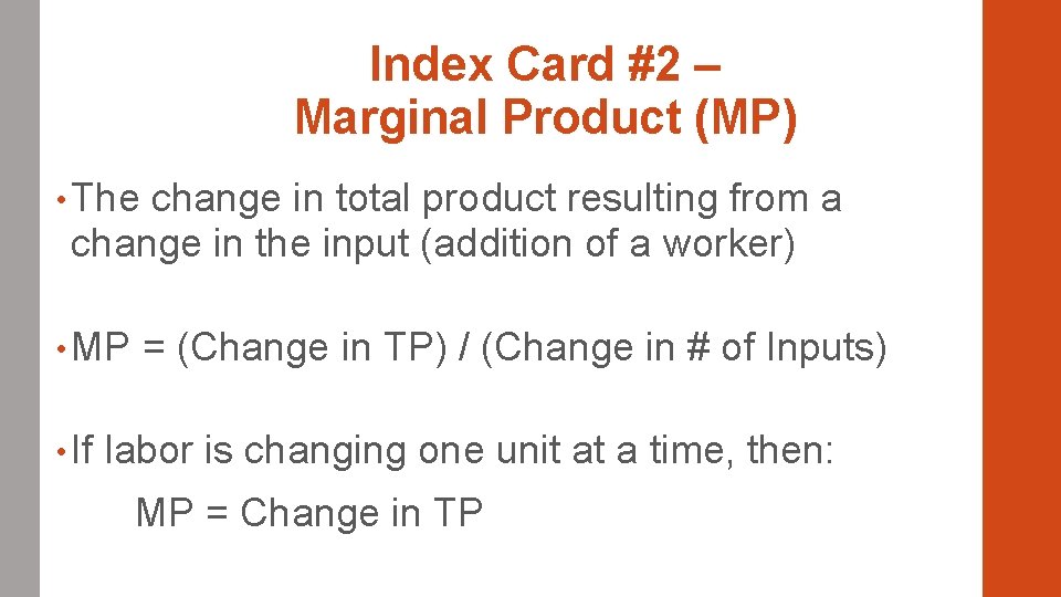
Index Card #2 – Marginal Product (MP) • The change in total product resulting from a change in the input (addition of a worker) • MP • If = (Change in TP) / (Change in # of Inputs) labor is changing one unit at a time, then: MP = Change in TP

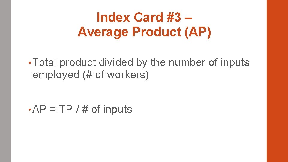
Index Card #3 – Average Product (AP) • Total product divided by the number of inputs employed (# of workers) • AP = TP / # of inputs

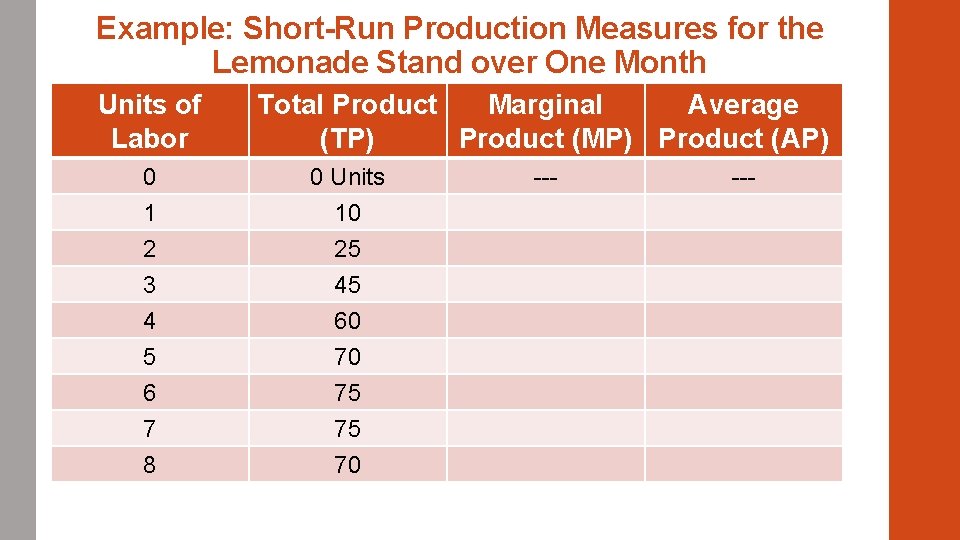
Example: Short-Run Production Measures for the Lemonade Stand over One Month Units of Labor Total Product Marginal Average (TP) Product (MP) Product (AP) 0 1 0 Units 10 2 3 4 5 25 45 60 70 6 7 8 75 75 70 ---

Graph the TP, MP, and AP data from the previous slide. (This is the last slide of day 1. ) • Locate the point where the MP & AP curves intersect. What do you notice about this point of intersection? • Look at the marginal product curve as the quantity of inputs increases. What can be said about the change in MP as outputs increase? • Why do you think MP changes the way you observed in the previous question?

Law of Diminishing Marginal Returns (1 st slide of day 2) ØAs successive units of a variable resource are added to a fixed resource, the additional output will eventually decrease. ØIt is not always more efficient to add more inputs, as we learned in the tennis ball game!

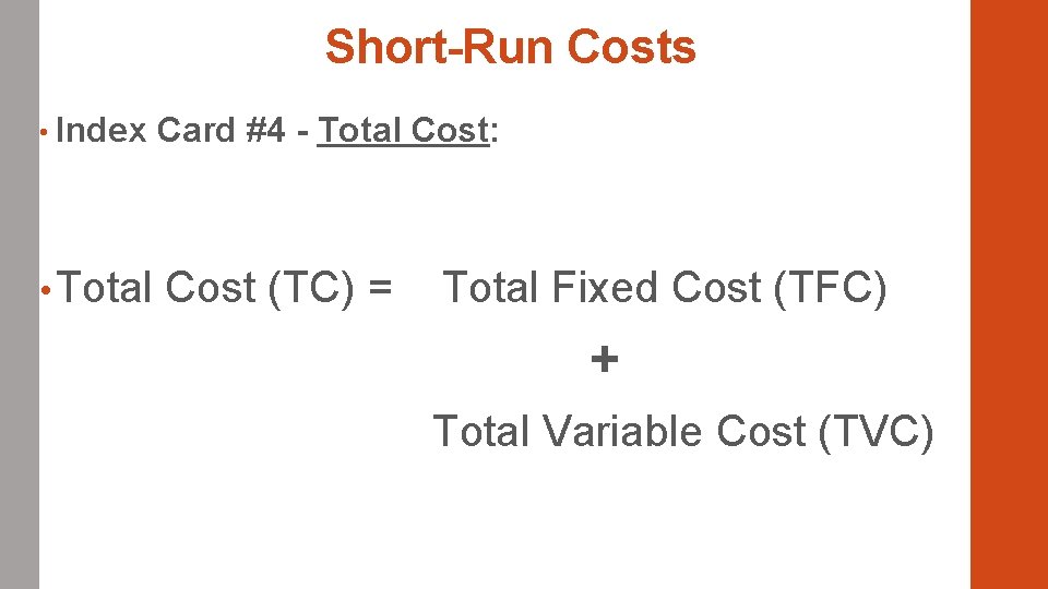
Short-Run Costs • Index Card #4 - Total Cost: • Total Cost (TC) = Total Fixed Cost (TFC) + Total Variable Cost (TVC)

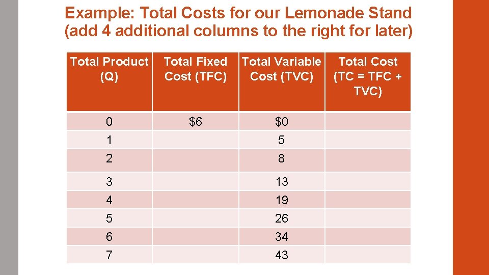
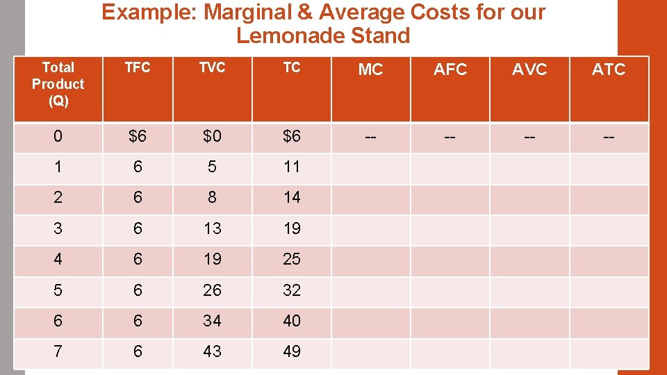
Example: Total Costs for our Lemonade Stand (add 4 additional columns to the right for later) Total Product (Q) Total Fixed Cost (TFC) 0 1 2 $6 3 4 5 6 7 Total Variable Total Cost (TVC) (TC = TFC + TVC) $0 5 8 13 19 26 34 43

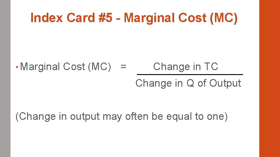
Index Card #5 - Marginal Cost (MC) • Marginal Cost (MC) = Change in TC Change in Q of Output (Change in output may often be equal to one)

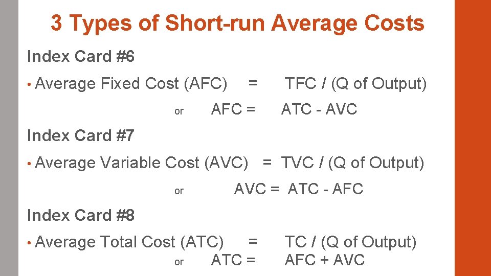
3 Types of Short-run Average Costs Index Card #6 • Average Fixed Cost (AFC) or = AFC = TFC / (Q of Output) ATC - AVC Index Card #7 • Average Variable Cost (AVC) = TVC / (Q of Output) AVC = ATC - AFC or Index Card #8 • Average Total Cost (ATC) or = ATC = TC / (Q of Output) AFC + AVC

Example: Marginal & Average Costs for our Lemonade Stand Total Product (Q) TFC TVC TC MC AFC AVC ATC 0 $6 $0 $6 -- -- 1 6 5 11 2 6 8 14 3 6 13 19 4 6 19 25 5 6 26 32 6 6 34 40 7 6 43 49

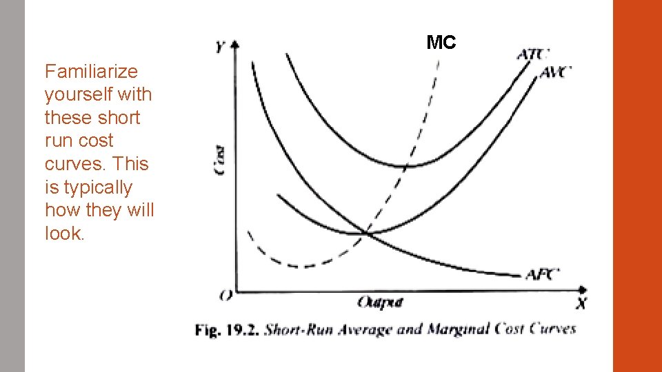
MC Familiarize yourself with these short run cost curves. This is typically how they will look.

Short-run & Long-run Decisions • Short run: a time period when at least one production input (plant size) is fixed and cannot be changed to respond to a change in product demand • Long run: a time period that is the amount of time required to change the plant size.

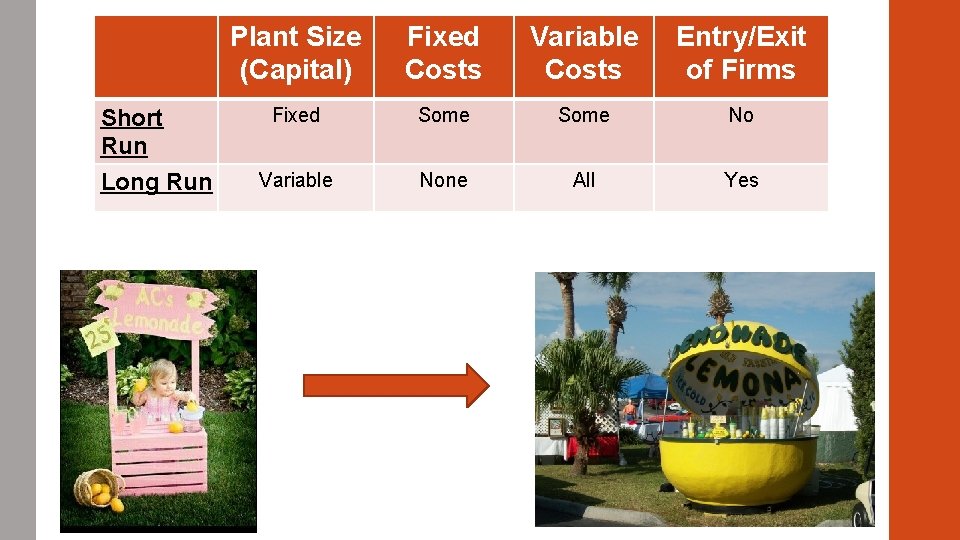
Short Run Long Run Plant Size (Capital) Fixed Costs Variable Costs Entry/Exit of Firms Fixed Some No Variable None All Yes

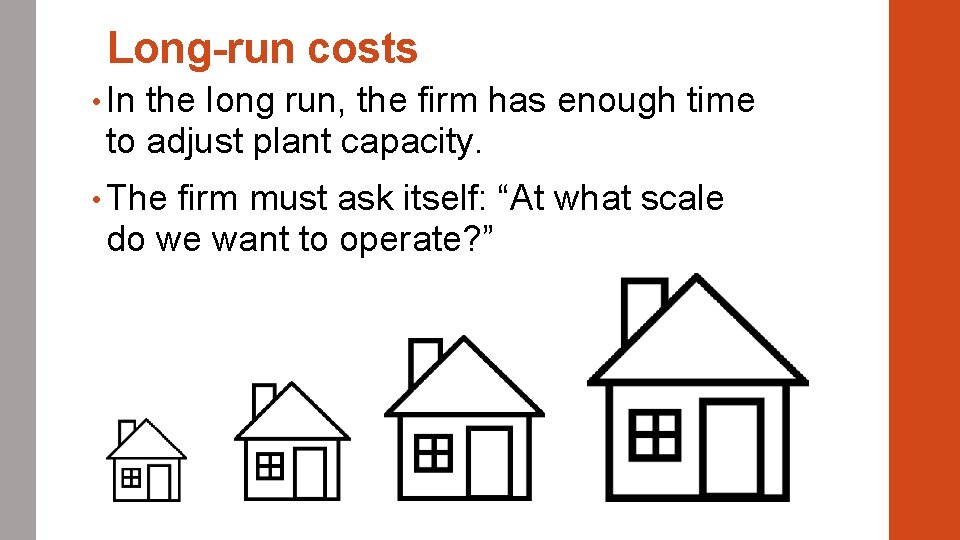
Long-run costs • In the long run, the firm has enough time to adjust plant capacity. • The firm must ask itself: “At what scale do we want to operate? ”

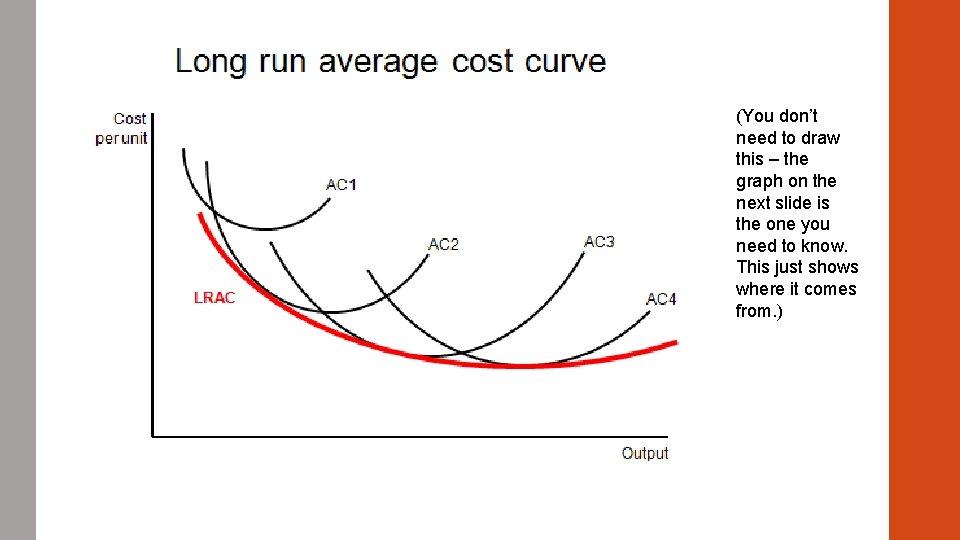
• Short-run average cost curves are snapshots of the firm’s ability to produce efficiently at the fixed plant size. • If we put these SRAC curves together, we can see a more continuous picture of the firm’s average costs.

(You don’t need to draw this – the graph on the next slide is the one you need to know. This just shows where it comes from. )

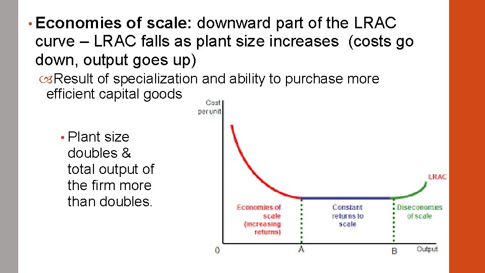
• Economies of scale: downward part of the LRAC curve – LRAC falls as plant size increases (costs go down, output goes up) Result of specialization and ability to purchase more efficient capital goods • Plant size doubles & total output of the firm more than doubles.

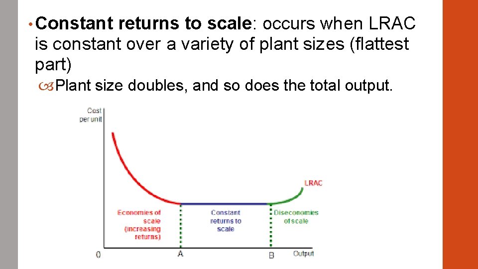
• Constant returns to scale: occurs when LRAC is constant over a variety of plant sizes (flattest part) Plant size doubles, and so does the total output.

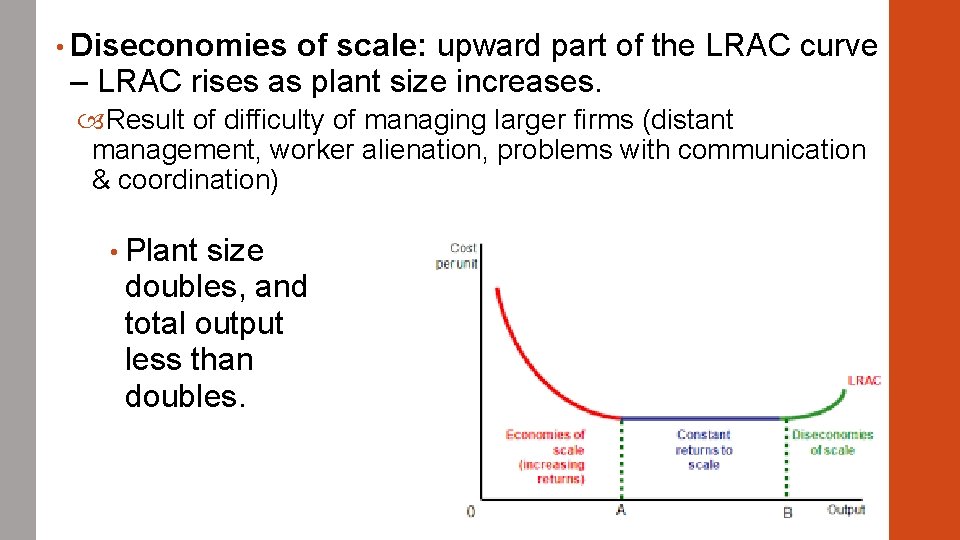
• Diseconomies of scale: upward part of the LRAC curve – LRAC rises as plant size increases. Result of difficulty of managing larger firms (distant management, worker alienation, problems with communication & coordination) • Plant size doubles, and total output less than doubles.