Process Control CHAPTER III LAPLACE TRANSFORM l The

Process Control CHAPTER III LAPLACE TRANSFORM

l The Laplace transform of a function f(t) is defined as; l In the application of Laplace transform variable time is eliminated and a new domain is introduced. In the modeling of dynamic systems differential equations are solved by using Laplace transform. l

Properties of Laplace Transform 1. 2. a. b. The Laplace transform contains no information about f(t) for t<0. (Since t represents time this is not a limitation) Laplace transform is defined with an improper integral. Therefore the required conditions are the function f(t) should be piecewise continuous the integral should have a finite value; i. e. , the function f(t) does not increase with time faster than e -st decreases with time.

3. 4. 5. Laplace transform operator transforms a function of variable t to a function of variable s. e. g. , T(t) becomes T(s) The Laplace transform is a linear operator. Tables for Laplace transforms are available. In those tables inverse transforms are also given.

Transforms of Some Functions 1. The constant function

2. The Step function

3. The exponential function

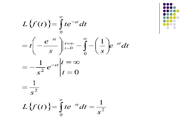
4. The Ramp function

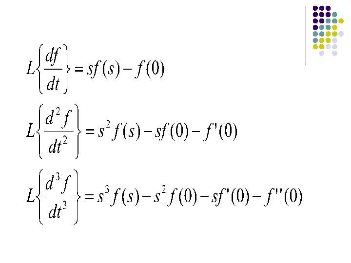
Laplace Transforms of Derivatives

Solution of Differential equations by Laplace Transform l l 1. 2. 3. For the solution of linear, ordinary differential equations with constant coefficients Laplace Transforms are applied. The procedure involves: Take the Laplace Transform of both sides of the equation. Solve the resulting equation for the Laplace transform of the unknown function. i. e. , evaluate x(s). Find the function x(t), which has the Laplace Transform obtained in step 2.

Example: l Solve the following equation. Solution:

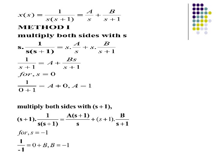
Inversion by Partial Fractions Example l Solve the following equation. Solution: Partial fractions is to be applied;

(by using Laplace Transform table)

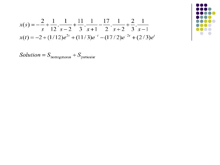
Example l Solve the following equation. Apply Laplace transform to both sides of the equation.

to determine multiply by Set s to results A S 0 -2 B S-2 2 1/12 C S+1 -1 11/3 D S+2 -2 -17/2 E S-1 1 2/3

Example Solve the following equation;

Example; l Find the solution of the equation with given laplace transform.

Example; Solve the following equation.

to multiply by determine A S Set s to results 0 1/6 B S+1 -1 -1/2 C S+2 -2 1/2 D S+3 -3 1/6

Example (Repeated factors) Solve the equation for which Laplace transform is given. Heaviside expansion rule can not be used for A, because the denominator of coefficient B becomes infinity.

Equalizing the derivatives gives Taking derivative w. r. t. s gives Further differentiation gives

Final Value Theorem Initial Value Theorem Transform of an integral

Example: Solve the following equation for x(t)

Example: l For a mixing tank, evaluate the change of composition w. r. t. time due to a step change in composition. w 1 x 1 w x (Overflow system with constant volume, having a component balance)

Example: l Considering Ex. 2. 1 for a sudden change in one of the input flow rates, evaluate concentration change w. r. t. time. Total mass balance; w 1, x 1 w 2 , x 2 w, x Component balance

For constant V and ρ ;

Example: Consider a CSTR and evaluate concentration change with respect to time.