Problem 1 Service System Capacity Queue Customers Server

Problem 1: Service System Capacity Queue Customers Server Served Customers Problem: Can a server taking an average of x time units meet the demand? Solution with an Analytical Model: Must specify the conditions on customer arrival, service completions. Take measurements or adopt assumptions (clearly specified). 1. Pr{customer arrives in interval (t, t + t]} = t + o( t) independent of t 2. Pr{service completes in interval (t, t + t]} = t + o( t) independent of t 3. Customer arrivals and service completions are mutually independent events 4. Population of customers is large and service is in order of arrival 5. The limit of the ratio o( t) / t as t 0 is 0

Analytical Model of Server Capacity Let pn(t) = Pr{n customers in the system at time t} Then pn(t + t) = pn-1(t) [ t + o( t)] + pn(t) [1 - t + o( t)] + pn+1(t) [ t + o( t)] n 1 P 0(t + t) = p 0(t) [1 - t + o( t)] + p 1(t) [ t + o( t)] Producing the steady-state equations: pn+1 – ( + ) pn + pn-1 = 0 (n 1) and p 1 - p 0 = 0 (n = 0) Solving for pn in terms of p 0 gives pn = ( / )n p 0 Using the fact that pn = 1 and letting = / , we obtain pn = n(1 - ) where < 1

Problem 1 Given a high-resolution computer image of a map of an irregularly shaped lake with several islands, determine the water surface area. Assume that the x-y coordinates of every point on the map can be measured at an acceptable level of resolution. Suggest alternative solution approaches!

Monte Carlo Simulation Y 0 Step 1: Enclose the area of interest in the smallest rectangle of known dimensions X and Y. Set j = 1, S = 0, and choose a large value for N where: j = trial number S = number of trials resulting in a hit on the water surface area N = total number of trials X

Monte Carlo Simulation Y RN y 0 RN x X Step 2: Generate a uniformly distributed random number, RNx over the length of X. Step 3: Generate another uniformly distributed random number, RNy over the length of Y.

Monte Carlo Simulation Y RN y 0 RN x Step 4: If the point of intersection, (RNx , RNy), falls on the water surface area, add 1 to S. Step 5: Add 1 to j. If j > N, go to Step 6; otherwise, go to Step 2. X

Monte Carlo Simulation Y RN y 0 Step 6: The estimate of the water surface area, A, is given by: NOTE: X RN x As N , A true value of the area A XY = S N

Problem 2 Use the fundamental theory and logic of the Monte Carlo Simulation technique to estimate the area under the Sine curve over 0 and . y 1 Sin (x) 0

Monte Carlo Simulation y 1 Sin (x) 0 Step 1: Enclose the area of interest in the smallest rectangle of known dimensions and 1. Set j = 1, S = 0, and choose a large value for N where: j = trial number S = number of trials with a hit on the area under the Sin (x) curve N = total number of trials

Monte Carlo Simulation y 1 RNy Sin (x) 0 RNx Step 2: Generate a uniformly distributed random number, RNx over the length of . Step 3: Generate another uniformly distributed random number, RNy over the length of 1.
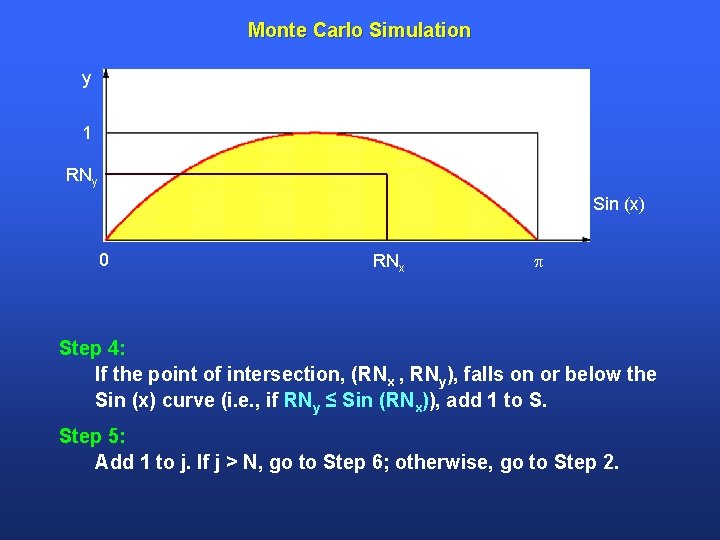
Monte Carlo Simulation y 1 RNy Sin (x) 0 RNx Step 4: If the point of intersection, (RNx , RNy), falls on or below the Sin (x) curve (i. e. , if RNy ≤ Sin (RNx)), add 1 to S. Step 5: Add 1 to j. If j > N, go to Step 6; otherwise, go to Step 2.
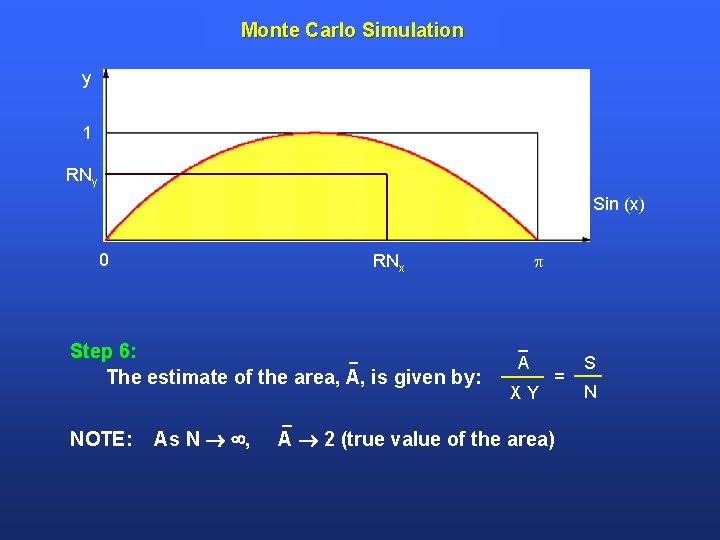
Monte Carlo Simulation y 1 RNy Sin (x) 0 Step 6: The estimate of the area, A, is given by: NOTE: RNx As N , A XY = A 2 (true value of the area) S N

Problem 3 Use the fundamental theory and logic of the Monte Carlo Simulation technique to solve the following optimization problem: Maximize Subject to: Z = ( e. X 1 + X 2 ) 2 + 3 ( 1 – X 3 ) 2 0 ≤ X 1 ≤ 1 0 ≤ X 2 ≤ 2 2 ≤ X 3 ≤ 3

Monte Carlo Simulation Use the fundamental theory and logic of the Monte Carlo Simulation technique to solve the following optimization problem: Maximize Subject to: Z = ( e. X 1 + X 2 ) 2 + 3 ( 1 – X 3 ) 2 0 ≤ X 1 ≤ 1 0 ≤ X 2 ≤ 2 2 ≤ X 3 ≤ 3 Step 1: Set j = 1 and choose a large value for N where: j = trial number N = total number of trials
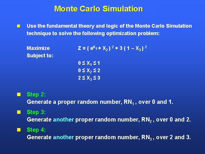
Monte Carlo Simulation Use the fundamental theory and logic of the Monte Carlo Simulation technique to solve the following optimization problem: Maximize Subject to: Z = ( e. X 1 + X 2 ) 2 + 3 ( 1 – X 3 ) 2 0 ≤ X 1 ≤ 1 0 ≤ X 2 ≤ 2 2 ≤ X 3 ≤ 3 Step 2: Generate a proper random number, RN 1 , over 0 and 1. Step 3: Generate another proper random number, RN 2 , over 0 and 2. Step 4: Generate another proper random number, RN 3 , over 2 and 3.
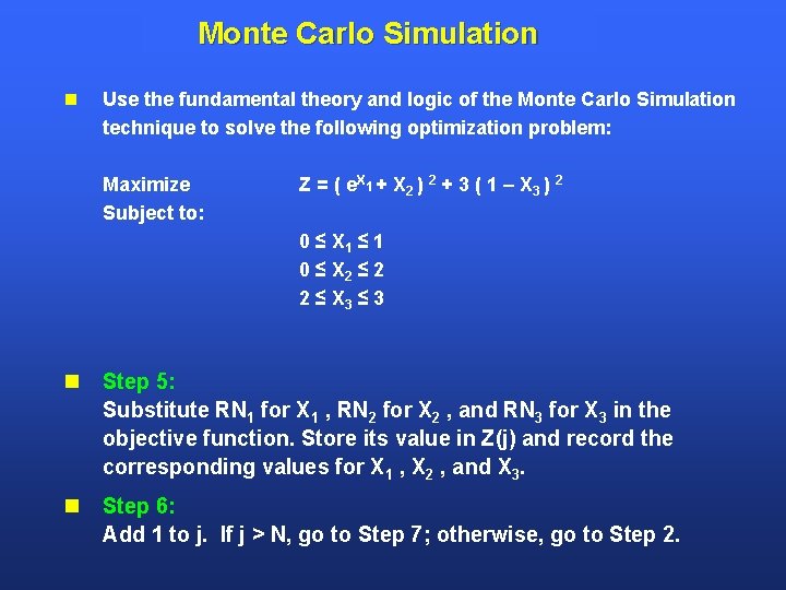
Monte Carlo Simulation Use the fundamental theory and logic of the Monte Carlo Simulation technique to solve the following optimization problem: Maximize Subject to: Z = ( e. X 1 + X 2 ) 2 + 3 ( 1 – X 3 ) 2 0 ≤ X 1 ≤ 1 0 ≤ X 2 ≤ 2 2 ≤ X 3 ≤ 3 Step 5: Substitute RN 1 for X 1 , RN 2 for X 2 , and RN 3 for X 3 in the objective function. Store its value in Z(j) and record the corresponding values for X 1 , X 2 , and X 3. Step 6: Add 1 to j. If j > N, go to Step 7; otherwise, go to Step 2.

Monte Carlo Simulation Use the fundamental theory and logic of the Monte Carlo Simulation technique to solve the following optimization problem: Maximize Subject to: Z = ( e. X 1 + X 2 ) 2 + 3 ( 1 – X 3 ) 2 0 ≤ X 1 ≤ 1 0 ≤ X 2 ≤ 2 2 ≤ X 3 ≤ 3 Step 7: The approximate solution of the problem is determined by the values of X 1 ( = RN 1 ), X 2 ( = RN 2 ), and X 3 ( = RN 3 ), which correspond to the maximum value of { Z(j), j = 1, 2, 3, . . . , N }. NOTE: As N , X 1 1, X 2 2, and X 3 3.
- Slides: 17