Probability Theory for Networking Application ECECSC 777 Telecommunications

Probability Theory for Networking Application ECE/CSC 777: Telecommunications Network Design Fall, 2013, Rudra Dutta

Why Probability ? l Extensive use in modeling networks traffic – Randomness exists - must deal with it Area of mathematics highly related to computer networking l Leads on to more powerful analysis tools and modeling paradigms l Markov chains – Queuing theory – Copyright Rudra Dutta, NCSU, Fall, 2013

Probability Formalization of “likelihood” of an event l Event space l “Equally likely” events l Ratio of event counts to total l Zero indicates impossibility – One indicates certainty – l Total probability – l Classical definition (more rigorous later) – l Some outcome must occur, so total of all probabilities must be 1 Classical definition needs a stretch to fit continuous case Ultimately, an element of “faith” or “trust” in nature Copyright Rudra Dutta, NCSU, Fall, 2013

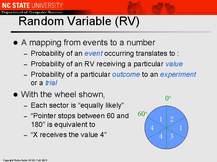
Random Variable (RV) l A mapping from events to a number Probability of an event occurring translates to : – Probability of an RV receiving a particular value – Probability of a particular outcome to an experiment or a trial – l With the wheel shown, Each sector is “equally likely” – “Pointer stops between 60 and 180” is equivalent to – “X receives the value 4” 0 o – Copyright Rudra Dutta, NCSU, Fall, 2013 60 o 1 2 4 1 4 3

Introductory Concepts l l l Distribution Expectation Conditional Probability Independent Events Memoryless RVs Copyright Rudra Dutta, NCSU, Fall, 2013

Probability Functions l Functions mapping value of an RV (outcome of a trial) to the probability of it occurring Discrete (finite or infinite) set of outcome described by probability mass function – Continuous set of outcomes described by probability density function – Sometime both are called density function – l Cumulative Density/Mass Function Adding up probability over successive outcomes – Sometimes called Probability Distribution Function – l Range of RV is the domain of P [. ] Copyright Rudra Dutta, NCSU, Fall, 2013

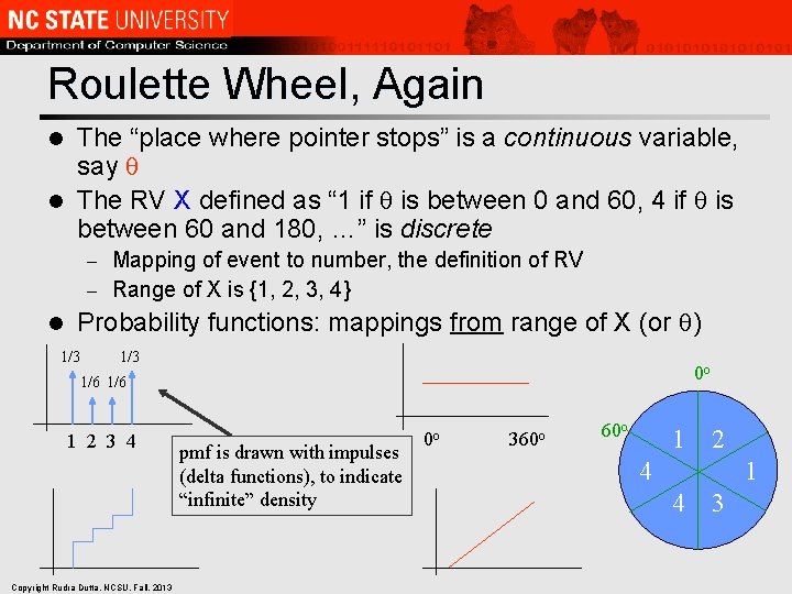
Roulette Wheel, Again The “place where pointer stops” is a continuous variable, say l The RV X defined as “ 1 if is between 0 and 60, 4 if is between 60 and 180, …” is discrete l Mapping of event to number, the definition of RV – Range of X is {1, 2, 3, 4} – l Probability functions: mappings from range of X (or ) 1/3 0 o 1/6 1 2 3 4 Copyright Rudra Dutta, NCSU, Fall, 2013 pmf is drawn with impulses (delta functions), to indicate “infinite” density 0 o 360 o 1 2 4 1 4 3

Combining Probability l Probabilities can be added for mutually exclusive events P [X is even] = 0. 5 – P [X is less than 4] = 2/3 – 1/3 0 o 1/6 1 2 3 4 Copyright Rudra Dutta, NCSU, Fall, 2013 pmf is drawn with impulses (delta functions), to indicate “infinite” density 0 o 360 o 1 2 4 1 4 3

PMF, PDF, PMF as PDF, CDF l PMF indicates actual probability at specific points – l PDF indicates rate at which probability is accumulated (hence: density) – l Derivative of probability (also a pure number!) Amassed probability (PMF) can be indicated on a PDF – l Probability is a pure (dimensionless) number (ratio of event counts) But must resort to “infinite” densities (impulses) CDF is integral of PDF, so indicates actual (cumulative) probabilities at each point) Copyright Rudra Dutta, NCSU, Fall, 2013

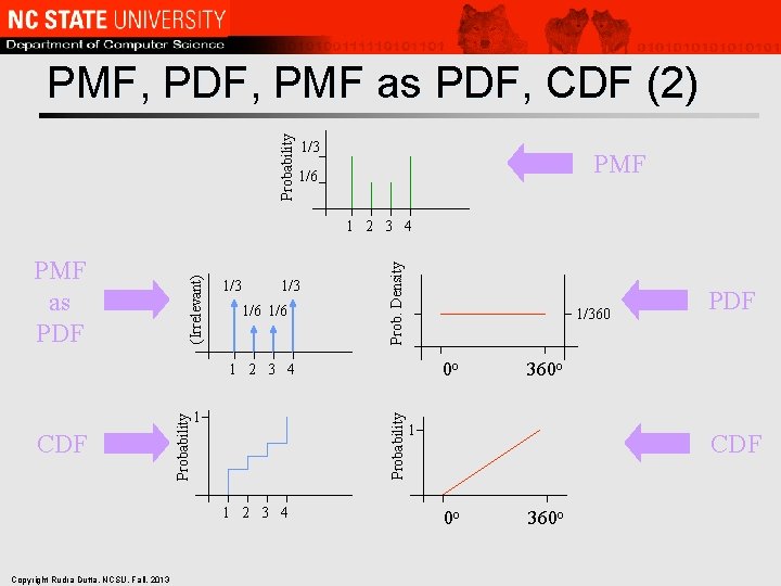
Probability PMF, PDF, PMF as PDF, CDF (2) 1/3 PMF 1/6 1/3 1/6 Prob. Density PMF as PDF (Irrelevant) 1 2 3 4 1/360 0 o 1 Probability CDF Probability 1 2 3 4 Copyright Rudra Dutta, NCSU, Fall, 2013 PDF 360 o 1 CDF 0 o 360 o

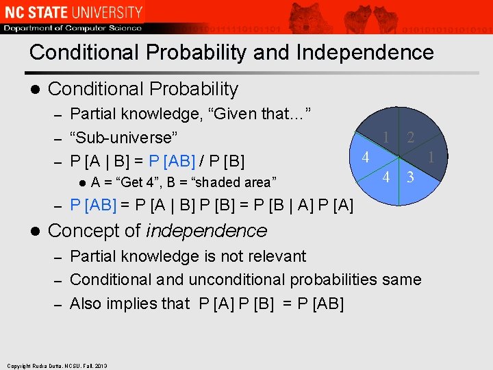
Conditional Probability and Independence l Conditional Probability Partial knowledge, “Given that…” – “Sub-universe” – P [A | B] = P [AB] / P [B] – l A = “Get 4”, B = “shaded area” 1 2 4 1 4 3 P [AB] = P [A | B] P [B] = P [B | A] P [A] Concept of independence Partial knowledge is not relevant – Conditional and unconditional probabilities same – Also implies that P [A] P [B] = P [AB] – Copyright Rudra Dutta, NCSU, Fall, 2013

Total Probability l Sum of conditional probabilities of an event For an exhaustive set of mutually exclusive events – Equals total probability of the original event 1 2 4 1 n 4 3 P [B] = S P [Ai. B] – i=1 P [Ai. B] = P [Ai | B] P [B] = P [B | Ai] P [Ai] n P [B] = S P [B | Ai] P [Ai] i=1 Bayes’ Theorem: n P [Ak | B] = P [Ak. B] / P [B] = P [B | Ak] P [Ak] / S P [B | Ai] P [Ai] i=1 Copyright Rudra Dutta, NCSU, Fall, 2013

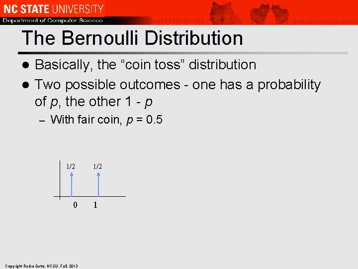
The Bernoulli Distribution Basically, the “coin toss” distribution l Two possible outcomes - one has a probability of p, the other 1 - p l – With fair coin, p = 0. 5 1/2 0 Copyright Rudra Dutta, NCSU, Fall, 2013 1/2 1

The Geometric Distribution “Try until a specific outcome” experiment on a event with Bernoulli distribution l For example, consider the coin toss l Keep tossing until you get Heads – Value of RV = number of tosses it took – One trial of this RV involves multiple trials of Bernoulli RV – l What is the probability distribution of this RV? – Key concept - each coin toss is independent Copyright Rudra Dutta, NCSU, Fall, 2013

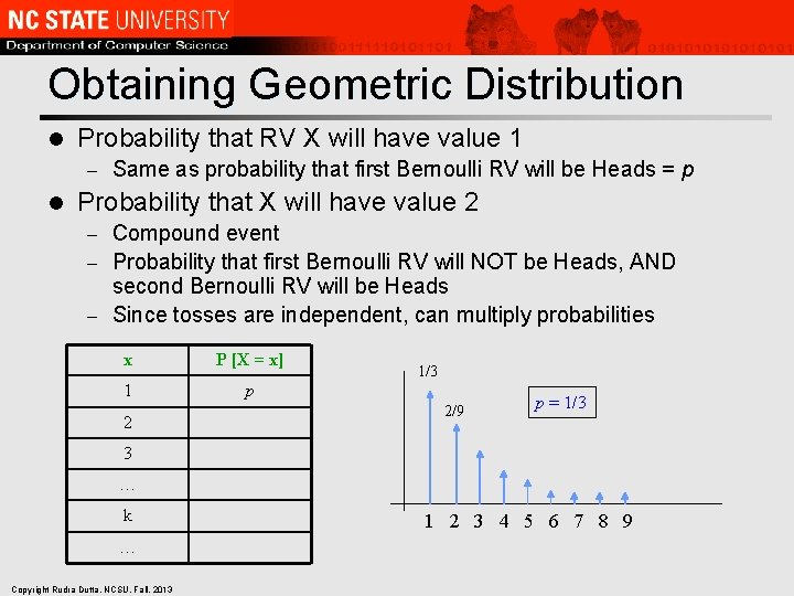
Obtaining Geometric Distribution l Probability that RV X will have value 1 – l Same as probability that first Bernoulli RV will be Heads = p Probability that X will have value 2 Compound event – Probability that first Bernoulli RV will NOT be Heads, AND second Bernoulli RV will be Heads – Since tosses are independent, can multiply probabilities – x P [X = x] 1 p 2 1/3 2/9 p = 1/3 3 … k … Copyright Rudra Dutta, NCSU, Fall, 2013 1 2 3 4 5 6 7 8 9

The Binomial Distribution The “k out of n” distribution l Flip n coins, RV is the number of Heads l – l It does not matter whether coins are tossed simultaneously or in sequence (or one coin n times) Probability of the RV being 0 Compound event: Bernoulli RV 1 is Tails, and Bernoulli RV 2 is Tails, … – Easily, (1 -p)n – l Probability of RV being 1 Compounding of compound events – BRV 1 is Heads, and BRV 2 is Tails, and … – OR, BRV 1 is Tails, and BRV 2 is Heads, and … – OR … – l Probability of RV being 2 BRV 1 is Heads, and BRV 2 is Heads, and BRV 3 is Tails, and … – OR, BRV 1 is Heads, and BRV 2 is Tails, and BRV 3 is Heads, … – OR, … – Copyright Rudra Dutta, NCSU, Fall, 2013

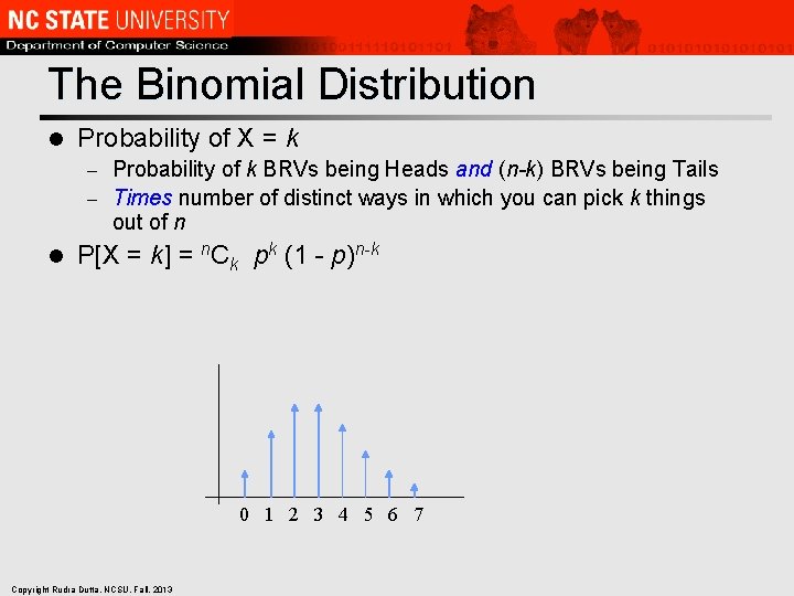
The Binomial Distribution l Probability of X = k Probability of k BRVs being Heads and (n-k) BRVs being Tails – Times number of distinct ways in which you can pick k things out of n – l P[X = k] = n. Ck pk (1 - p)n-k 0 1 2 3 4 5 6 7 Copyright Rudra Dutta, NCSU, Fall, 2013

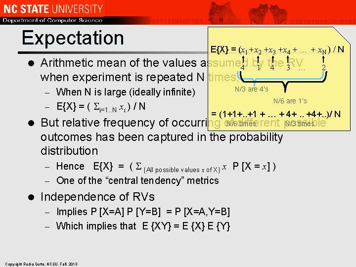
Expectation l E{X} = (x 1+x 2 +x 3 +x 4 + … + x. N ) / N Arithmetic mean of the values assumed 4 by 1 the 4 3 RV … when experiment is repeated N times, When N is large (ideally infinite) – E{X} = ( Si=1. . N xi ) / N N/3 are 4’s – l N/6 are 1’s = (1+1+. . +1 + … + 4+. . +4+. . )/ N N/6 different times N/3 times But relative frequency of occurring of possible outcomes has been captured in the probability distribution Hence E{X} = ( S {All possible values x of X} x P [X = x] ) – One of the “central tendency” metrics – l 2 Independence of RVs Implies P [X=A] P [Y=B] = P [X=A, Y=B] – Which implies that E {XY} = E {X} E {Y} – Copyright Rudra Dutta, NCSU, Fall, 2013

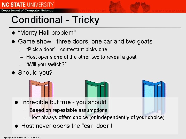
Conditional - Tricky “Monty Hall problem” l Game show - three doors, one car and two goats l “Pick a door” - contestant picks one – Host opens one of the other two to reveal a goat – “Will you switch? ” – l l Should you? Incredible but true - you should Based on repeatable assumptions – Host always offers choice (or independently of your choice) – l Host never opens the “car” door ! Copyright Rudra Dutta, NCSU, Fall, 2013

Conditioning and Memorylessness Successive values (discrete) or intervals (continuous) of domain of P[. ] can be looked upon as a sequence l Memory – refers to special type of conditioning l “RV is greater than x ” – In sequence terms: “has survived x ” – If this conditioning has no effect memoryless – Key observation: independence in successive trials translates to memorylessness in distribution l Geometric distribution l Continuous analogue – exponential distribution: f(x) = e - x l p p (1 -p) 1 2 3 4 5 6 7 8 9 Copyright Rudra Dutta, NCSU, Fall, 2013 1 2 3 4 5 6 7 8 9

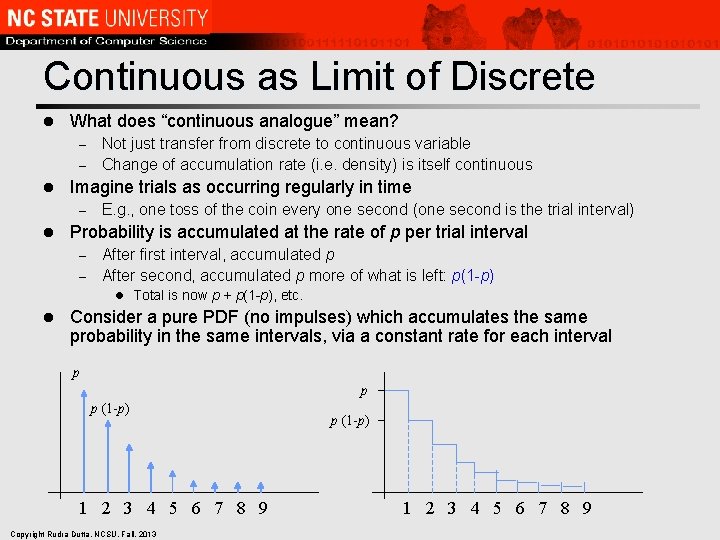
Continuous as Limit of Discrete l What does “continuous analogue” mean? Not just transfer from discrete to continuous variable – Change of accumulation rate (i. e. density) is itself continuous – l Imagine trials as occurring regularly in time – l E. g. , one toss of the coin every one second (one second is the trial interval) Probability is accumulated at the rate of p per trial interval After first interval, accumulated p – After second, accumulated p more of what is left: p(1 -p) – l Total is now p + p(1 -p), etc. l Consider a pure PDF (no impulses) which accumulates the same probability in the same intervals, via a constant rate for each interval p p p (1 -p) 1 2 3 4 5 6 7 8 9 Copyright Rudra Dutta, NCSU, Fall, 2013 p (1 -p) 1 2 3 4 5 6 7 8 9

Focus on Change in Rate l Now we have a distribution for a continuous experiment (variable) The outcome can be any real value, 0 or 1, also 1. 5, 1. 25, 0. 9999, etc. – For each of these, probability accumulates at a rate or density which itself goes down in steps – At each step, the rate is such that a fixed fraction (p) of the remaining probability is accumulated in the next interval – l Consider making the steps finer, eventually infinitesimal Now the rate goes down continuously – But at each infinitesimal interval, the fraction of remaining probability accumulated is the same – l The memoryless property is preserved Copyright Rudra Dutta, NCSU, Fall, 2013

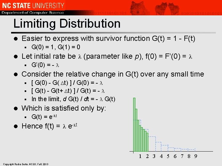
Limiting Distribution l Easier to express with survivor function G(t) = 1 - F(t) § l Let initial rate be (parameter like p), f(0) = F’(0) = § l G(0) = 1, G(1) = 0 G’(0) = - Consider the relative change in G(t) over any small time [ G(0) - G( t) ] / G(0) = - § [ G(t) - G(t+ t) ] / G(t) = - § In the limit, d G(t) / dt = - G(t) § l Which is satisfied only by: § l G(t) = e- t Hence f(t) = e- t 1 2 3 4 5 6 7 8 9 Copyright Rudra Dutta, NCSU, Fall, 2013

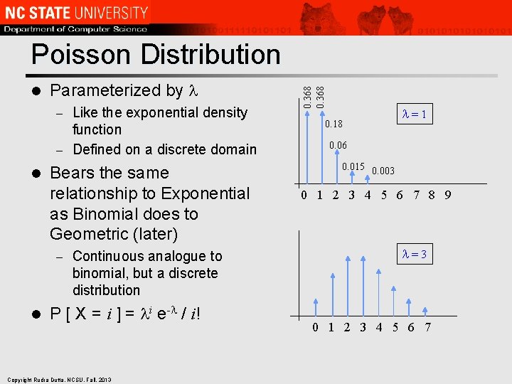
l Parameterized by Like the exponential density function – Defined on a discrete domain – l Bears the same relationship to Exponential as Binomial does to Geometric (later) – l Continuous analogue to binomial, but a discrete distribution P [ X = i ] = i e- / i! Copyright Rudra Dutta, NCSU, Fall, 2013 0. 368 Poisson Distribution 0. 18 =1 0. 06 0. 015 0. 003 0 1 2 3 4 5 6 7 8 9 =3 0 1 2 3 4 5 6 7

The Renewal Counting Paradigm Accumulated count of lifetimes is also of interest l The original variable denotes lifetime l – l The counting variable denotes total such lifetimes – l For packet transmission, time to transmit a single packet successfully For packet transmission, the number of packets transmitted successfully in a given time Ends of lifetimes are called renewals – Hence renewal counting Copyright Rudra Dutta, NCSU, Fall, 2013

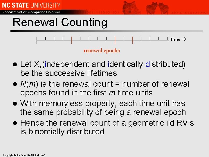
Renewal Counting time renewal epochs Let Xi (independent and identically distributed) be the successive lifetimes l N(m) is the renewal count = number of renewal epochs found in the first m time units l With memoryless property, each time unit has the same probability of being a renewal epoch l Hence the renewal count of a geometric iid RV’s is binomially distributed l Copyright Rudra Dutta, NCSU, Fall, 2013

Relevant Renewal Results l l l Geometric interarrival binomial arrival count Binomial arrival count geometric interarrival Exponential interarrival Poisson arrival count exponential interarrival Merging Poisson arrivals Poisson process Statistically splitting Poisson arrival into two arrival processes (using a Bernoulli variable for the splitting) Poisson resultant processes Copyright Rudra Dutta, NCSU, Fall, 2013

Probability Reference? l Many good texts Whatever you have used before may help – Following should work – But not “best” or “most useful” in any sense – l "Fundamentals of Applied Probability Theory” – l "Probability, Stochastic Processes, and queueing theory” – l by Drake by Nelson "Probability and random processes for electrical engineers” – by Viniotis Copyright Rudra Dutta, NCSU, Fall, 2013