Probability The definition probability of an Event Applies

Probability

The definition – probability of an Event Applies only to the special case when 1. The sample space has a finite no. of outcomes, and 2. Each outcome is equi-probable If this is not true a more general definition of probability is required.

Summary of the Rules of Probability
![The additive rule P[A B] = P[A] + P[B] – P[A B] and P[A](http://slidetodoc.com/presentation_image_h/279db538cba067b72a97dade9e9a9eee/image-4.jpg "The additive rule P[A B] = P[A] + P[B] – P[A B] and P[A")
The additive rule P[A B] = P[A] + P[B] – P[A B] and P[A B] = P[A] + P[B] if A B = f

The Rule for complements for any event E

Conditional probability

The multiplicative rule of probability and if A and B are independent. This is the definition of independent

Counting techniques
")
Summary of counting results Rule 1 n(A 1 A 2 A 3 …. ) = n(A 1) + n(A 2) + n(A 3) + … if the sets A 1, A 2, A 3, … are pairwise mutually exclusive (i. e. Ai Aj = f) Rule 2 N = n 1 n 2 = the number of ways that two operations can be performed in sequence if n 1 = the number of ways the first operation can be performed n 2 = the number of ways the second operation can be performed once the first operation has been completed.

Rule 3 N = n 1 n 2 … nk = the number of ways the k operations can be performed in sequence if n 1 = the number of ways the first operation can be performed ni = the number of ways the ith operation can be performed once the first (i - 1) operations have been completed. i = 2, 3, … , k

Basic counting formulae 1. Orderings 2. Permutations The number of ways that you can choose k objects from n in a specific order 3. Combinations The number of ways that you can choose k objects from n (order of selection irrelevant)

Applications to some counting problems • The trick is to use the basic counting formulae together with the Rules • We will illustrate this with examples • Counting problems are not easy. The more practice better the techniques

Random Variables Numerical Quantities whose values are determine by the outcome of a random experiment

Random variables are either • Discrete – Integer valued – The set of possible values for X are integers • Continuous – The set of possible values for X are all real numbers – Range over a continuum.

Examples • Discrete – A die is rolled and X = number of spots showing on the upper face. – Two dice are rolled and X = Total number of spots showing on the two upper faces. – A coin is tossed n = 100 times and X = number of times the coin toss resulted in a head. – We observe X, the number of hurricanes in the Carribean from April 1 to September 30 for a given year

Examples • Continuous – A person is selected at random from a population and X = weight of that individual. – A patient who has received who has revieved a kidney transplant is measured for his serum creatinine level, X, 7 days after transplant. – A sample of n = 100 individuals are selected at random from a population (i. e. all samples of n = 100 have the same probability of being selected). X = the average weight of the 100 individuals.

The Probability distribution of A random variable A Mathematical description of the possible values of the random variable together with the probabilities of those values

The probability distribution of a discrete random variable is describe by its : probability function p(x) = the probability that X takes on the value x. This can be given in either a tabular form or in the form of an equation. It can also be displayed in a graph.

Example 1 • Discrete – A die is rolled and X = number of spots showing on the upper face. x 1 2 3 4 5 6 p(x) 1/6 1/6 1/6 formula – p(x) = 1/6 if x = 1, 2, 3, 4, 5, 6
, draw bars of height p(x) above each")
Graphs To plot a graph of p(x), draw bars of height p(x) above each value of x. Rolling a die

Example 2 – Two dice are rolled and X = Total number of spots showing on the two upper faces. x p(x) 2 3 4 5 6 7 8 9 10 11 12 1/36 2/36 3/36 4/36 5/36 6/36 5/36 4/36 3/36 2/36 1/36 Formula:

Rolling two dice

36 possible outcome for rolling two dice

Comments: Every probability function must satisfy: 1. The probability assigned to each value of the random variable must be between 0 and 1, inclusive: 2. The sum of the probabilities assigned to all the values of the random variable must equal 1: 3.

Example In baseball the number of individuals, X, on base when a home run is hit ranges in value from 0 to 3. The probability distribution is known and is given below: Note: n This chart implies the only values x takes on are 0, 1, 2, and 3. n If the random variable X is observed repeatedly the probabilities, p(x), represents the proportion times the value x appears in that sequence. P ( the random variable X equals 2) = p (2) = 3 14

A Bar Graph

Discrete Random Variables Discrete Random Variable: A random variable usually assuming an integer value. • a discrete random variable assumes values that are isolated points along the real line. That is neighbouring values are not “possible values” for a discrete random variable Note: Usually associated with counting • The number of times a head occurs in 10 tosses of a coin • The number of auto accidents occurring on a weekend • The size of a family

Continuous Random Variables Continuous Random Variable: A quantitative random variable that can vary over a continuum • A continuous random variable can assume any value along a line interval, including every possible value between any two points on the line Note: Usually associated with a measurement • Blood Pressure • Weight gain • Height

Random Variables Numerical Quantities whose values are determine by the outcome of a random experiment

The probability distribution of a discrete random variable is describe by its : probability function p(x) = the probability that X takes on the value x. This can be given in either a tabular form or in the form of an equation. It can also be displayed in a graph.

Example

Probability Distributions of Continuous Random Variables

Probability Density Function The probability distribution of a continuous random variable is describe by probability density curve f(x).

Notes: n n The Total Area under the probability density curve is 1. The Area under the probability density curve is from a to b is P[a < X < b].
")
Normal Probability Distributions (Bell shaped curve)
 of a Discrete Probability Distribution • Describe the center")
Mean and Variance (standard deviation) of a Discrete Probability Distribution • Describe the center and spread of a probability distribution • The mean (denoted by greek letter m (mu)), measures the centre of the distribution. • The variance (s 2) and the standard deviation (s) measure the spread of the distribution. s is the greek letter for s.
 of a Probability Distribution")
Mean, Variance (and standard deviation) of a Probability Distribution

Mean of a Discrete Random Variable • The mean, m, of a discrete random variable x is found by multiplying each possible value of x by its own probability and then adding all the products together: Notes: n n n The mean is a weighted average of the values of X. The mean is the long-run average value of the random variable. The mean is centre of gravity of the probability distribution of the random variable

Variance and Standard Deviation Variance of a Discrete Random Variable: Variance, s 2, of a discrete random variable x is found by multiplying each possible value of the squared deviation from the mean, (x - m)2, by its own probability and then adding all the products together: Standard Deviation of a Discrete Random Variable: The positive square root of the variance: s = s 2

Example The number of individuals, X, on base when a home run is hit ranges in value from 0 to 3.

• Computing the mean: Note: • 0. 929 is the long-run average value of the random variable • 0. 929 is the centre of gravity value of the probability distribution of the random variable

• Computing the variance: • Computing the standard deviation:

Random Variables Numerical Quantities whose values are determine by the outcome of a random experiment

Random variables are either • Discrete – Integer valued – The set of possible values for X are integers • Continuous – The set of possible values for X are all real numbers – Range over a continuum.

The Probability distribution of A random variable A Mathematical description of the possible values of the random variable together with the probabilities of those values

The probability distribution of a discrete random variable is describe by its : probability function p(x) = the probability that X takes on the value x. This can be given in either a tabular form or in the form of an equation. It can also be displayed in a graph.

Example In baseball the number of individuals, X, on base when a home run is hit ranges in value from 0 to 3. The probability distribution is known and is given below: Note: n This chart implies the only values x takes on are 0, 1, 2, and 3. n If the random variable X is observed repeatedly the probabilities, p(x), represents the proportion times the value x appears in that sequence. P ( the random variable X equals 2) = p (2) = 3 14

A Bar Graph

Probability Distributions of Continuous Random Variables

Probability Density Function The probability distribution of a continuous random variable is describe by probability density curve f(x).

Notes: n n The Total Area under the probability density curve is 1. The Area under the probability density curve is from a to b is P[a < X < b].

Mean, Variance and standard deviation of Random Variables Numerical descriptors of the distribution of a Random Variable

Mean of a Discrete Random Variable • The mean, m, of a discrete random variable x is found by multiplying each possible value of x by its own probability and then adding all the products together: Notes: n n n The mean is a weighted average of the values of X. The mean is the long-run average value of the random variable. The mean is centre of gravity of the probability distribution of the random variable

Variance and Standard Deviation Variance of a Discrete Random Variable: Variance, s 2, of a discrete random variable x is found by multiplying each possible value of the squared deviation from the mean, (x - m)2, by its own probability and then adding all the products together: Standard Deviation of a Discrete Random Variable: The positive square root of the variance: s = s 2

Example The number of individuals, X, on base when a home run is hit ranges in value from 0 to 3.

• Computing the mean: Note: • 0. 929 is the long-run average value of the random variable • 0. 929 is the centre of gravity value of the probability distribution of the random variable

• Computing the variance: • Computing the standard deviation:

The Binomial distribution An important discrete distribution

Situation - in which the binomial distribution arises • We have a random experiment that has two outcomes – Success (S) and failure (F) – p = P[S], q = 1 - p = P[F], • The random experiment is repeated n times independently • X = the number of times S occurs in the n repititions • Then X has a binomial distribution

Example • A coin is tosses n = 20 times – X = the number of heads – Success (S) = {head}, failure (F) = {tail – p = P[S] = 0. 50, q = 1 - p = P[F]= 0. 50 • An eye operation has %85 chance of success. It is performed n =100 times – X = the number of Sucesses (S) – p = P[S] = 0. 85, q = 1 - p = P[F]= 0. 15 • In a large population %30 support the death penalty. A sample n =50 indiviuals are selected at random – X = the number who support the death penalty (S) – p = P[S] = 0. 30, q = 1 - p = P[F]= 0. 70
 and")
The Binomial distribution 1. We have an experiment with two outcomes – Success(S) and Failure(F). 2. Let p denote the probability of S (Success). 3. In this case q=1 -p denotes the probability of Failure(F). 4. This experiment is repeated n times independently. 5. X denote the number of successes occuring in the n repititions.

The possible values of X are 0, 1, 2, 3, 4, … , (n – 2), (n – 1), n and p(x) for any of the above values of x is given by: X is said to have the Binomial distribution with parameters n and p.

Summary: X is said to have the Binomial distribution with parameters n and p. 1. X is the number of successes occurring in the n repetitions of a Success-Failure Experiment. 2. The probability of success is p. 3. The probability function

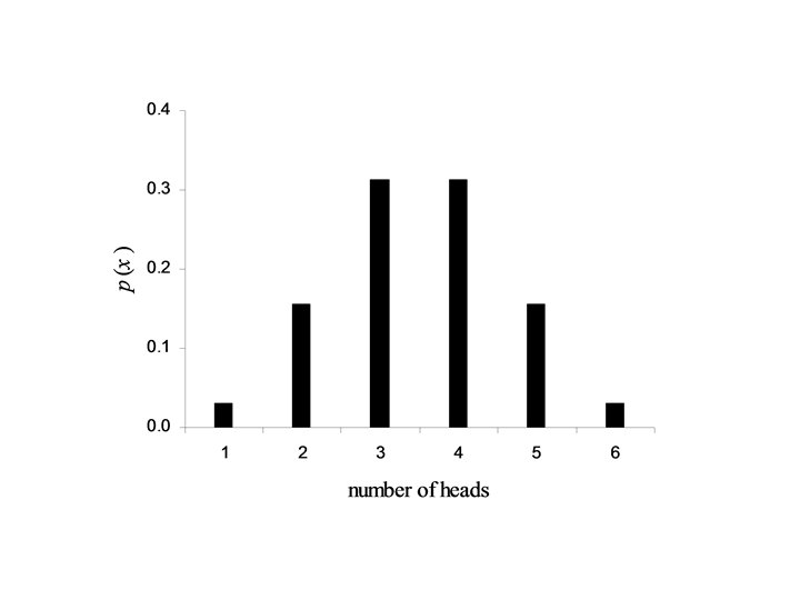
Example: 1. A coin is tossed n = 5 times. X is the number of heads occurring in the 5 tosses of the coin. In this case p = ½ and x p(x) 0 1 2 3 4 5

Note:

Computing the summary parameters for the distribution – m, s 2, s

• Computing the mean: • Computing the variance: • Computing the standard deviation:

Example: • A surgeon performs a difficult operation n = 10 times. • X is the number of times that the operation is a success. • The success rate for the operation is 80%. In this case p = 0. 80 and • X has a Binomial distribution with n = 10 and p = 0. 80.
 for x = 0, 1, 2, 3, … , 10")
Computing p(x) for x = 0, 1, 2, 3, … , 10

The Graph

Computing the summary parameters for the distribution – m, s 2, s

• Computing the mean: • Computing the variance: • Computing the standard deviation:

Notes n n n The value of many binomial probabilities are found in Tables posted on the Stats 244 site. The value that is tabulated for n = 1, 2, 3, …, 20; 25 and various values of p is: Hence n The other table, tabulates p(x). Thus when using this table you will have to sum up the values

Example n n n Suppose n = 8 and p = 0. 70 and we want to compute P[X = 5] = p(5) Table value for n = 8, p = 0. 70 and c =5 is 0. 448 = P[X ≤ 5] P[X = 5] = p(5) = P[X ≤ 5] - P[X ≤ 4] = 0. 448 – 0. 194 =. 254
")
We can also compute Binomial probabilities using Excel The function =BINOMDIST(x, n, p, FALSE) will compute p(x). The function =BINOMDIST(c, n, p, TRUE) will compute

Mean, Variance and standard deviation of Binomial Random Variables

Mean, Variance and standard deviation of Discrete Random Variables

Mean of a Discrete Random Variable • The mean, m, of a discrete random variable x Notes: n n n The mean is a weighted average of the values of X. The mean is the long-run average value of the random variable. The mean is centre of gravity of the probability distribution of the random variable

Variance and Standard Deviation Variance of a Discrete Random Variable: Variance, s 2, of a discrete random variable x Standard Deviation of a Discrete Random Variable: The positive square root of the variance: s = s 2

The Binomial distribution

The Binomial distribution X is said to have the Binomial distribution with parameters n and p. 1. X is the number of successes occurring in the n repetitions of a Success-Failure Experiment. 2. The probability of success is p. 3. The probability function

Mean, Variance & Standard Deviation of the Binomial Ditribution • The mean, variance and standard deviation of the binomial distribution can be found by using the following three formulas:

Example: Find the mean and standard deviation of the binomial distribution when n = 20 and p = 0. 75 Solutions: 1) n = 20, p = 0. 75, q = 1 - 0. 75 = 0. 25 m = np = (20)(0. 75) = 15 s = npq = (20)(0. 75)(0. 25) = 3. 75 » 1936. 2) These values can also be calculated using the probability function: æ 20ö p ( x ) = ç ÷ (0. 75) x (0. 25)20 x for x = 0, 1, 2, . . . , 20 è xø

Table of probabilities

• Computing the mean: • Computing the variance: • Computing the standard deviation:

Histogram m s

Probability Distributions of Continuous Random Variables

Probability Density Function The probability distribution of a continuous random variable is describe by probability density curve f(x).

Notes: n n The Total Area under the probability density curve is 1. The Area under the probability density curve is from a to b is P[a < X < b].
 • The mean, m, of a")
Mean of a Continuous Random Variable (uses calculus) • The mean, m, of a discrete random variable x Notes: n n n The mean is a weighted average of the values of X. The mean is the long-run average value of the random variable. The mean is centre of gravity of the probability distribution of the random variable

Variance and Standard Deviation Variance of a Continuous Random Variable: Variance, s 2, of a discrete random variable x Standard Deviation of a Discrete Random Variable: The positive square root of the variance: s = s 2

Normal Probability Distributions

Normal Probability Distributions • The normal probability distribution is the most important distribution in all of statistics • Many continuous random variables have normal or approximately normal distributions

The Normal Probability Distribution Points of Inflection

Main characteristics of the Normal Distribution • Bell Shaped, symmetric • Points of inflection on the bell shaped curve are at m – s and m + s. That is one standard deviation from the mean • Area under the bell shaped curve between m – s and m + s is approximately 2/3. • Area under the bell shaped curve between m – 2 s and m + 2 s is approximately 95%.

There are many Normal distributions depending on by m and s Normal m = 100, s =20 Normal m = 100, s = 40 Normal m = 140, s =20

The Standard Normal Distribution m = 0, s = 1
")
• There are infinitely many normal probability distributions (differing in m and s) • Area under the Normal distribution with mean m and standard deviation s can be converted to area under the standard normal distribution • If X has a Normal distribution with mean m and standard deviation s than has a standard normal distribution. • z is called the standard score (z-score) of X.

Converting Area under the Normal distribution with mean m and standard deviation s to Area under the standard normal distribution

Perform the z-transformation then Area under the Normal distribution with mean m and standard deviation s Area under the standard normal distribution

Area under the Normal distribution with mean m and standard deviation s s m

Area under the standard normal distribution 1 0

Using the tables for the Standard Normal distribution

Table, Posted on stats 245 web site • The table contains the area under the standard normal curve between -∞ and a specific value of z

Example Find the area under the standard normal curve between z = -∞ and z = 1. 45 • A portion of Table 3: z 0. 00 0. 01 0. 02 0. 03 0. 04 0. 05 . . . 1. 4. . . 0. 9265 0. 06
")
Example Find the area to the left of -0. 98; P(z < -0. 98) P ( z < - 0. 98) = 0. 1635

Example Find the area under the normal curve to the right of z = 1. 45; P(z > 1. 45)

Example Find the area to the between z = 0 and of z = 1. 45; P(0 < z < 1. 45) • Area between two points = differences in two tabled areas

Notes Use the fact that the area above zero and the area below zero is 0. 5000 n n n the area above zero is 0. 5000 When finding normal distribution probabilities, a sketch is always helpful
 and z = -1.")
Example: Find the area between the mean (z = 0) and z = -1. 26

Example: Find the area between z = -2. 30 and z = 1. 80

Example: Find the area between z = -1. 40 and z = -0. 50
 Approach: 1.")
Computing Areas under the general Normal Distributions (mean m, standard deviation s) Approach: 1. Convert the random variable, X, to its z-score. 2. Convert the limits on random variable, X, to their z-scores. 3. Convert area under the distribution of X to area under the standard normal distribution.

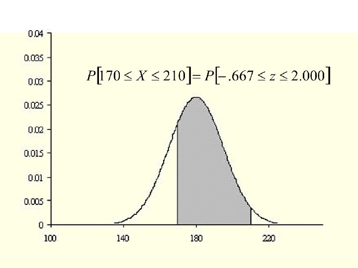
Example 1: Suppose a man aged 40 -45 is selected at random from a population. • X is the Blood Pressure of the man. • X is random variable. • Assume that X has a Normal distribution with mean m =180 and a standard deviation s = 15.

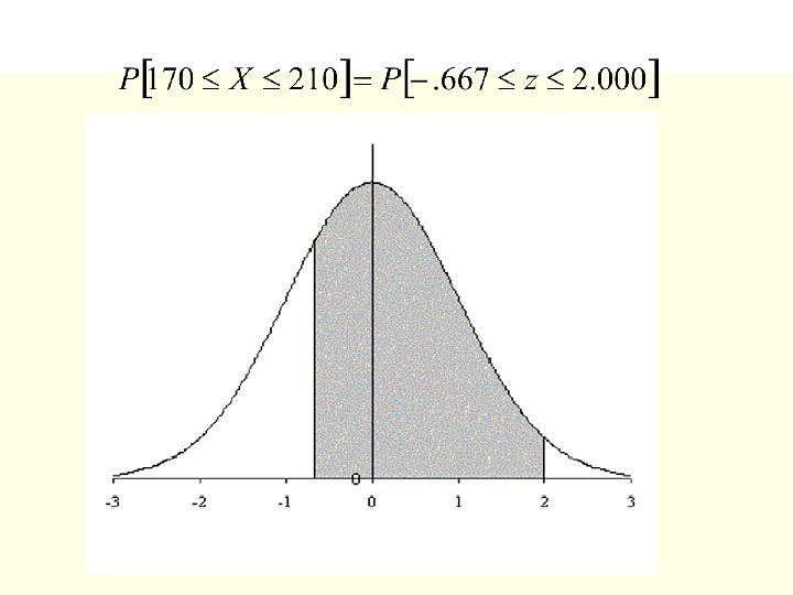
The probability density of X is plotted in the graph below. • Suppose that we are interested in the probability that X between 170 and 210.

Let Hence

Example 2 A bottling machine is adjusted to fill bottles with a mean of 32. 0 oz of soda and standard deviation of 0. 02. Assume the amount of fill is normally distributed and a bottle is selected at random: 1) Find the probability the bottle contains between 32. 00 oz and 32. 025 oz 2) Find the probability the bottle contains more than 31. 97 oz
 When x = 32. 00 When x = 32. 025")
Solution part 1) When x = 32. 00 When x = 32. 025

Graphical Illustration: 32. 0 - 32. 0 X - 32. 025 - 32. 0 ö æ < < ÷ P ( 32. 0 < X < 32. 025) = P ç è ø 0. 02 = P ( 0 < z < 1. 25) = 0. 3944
 x - 32. 0 3197. - 32. 0 ö æ")
Example 2, Part 2) x - 32. 0 3197. - 32. 0 ö æ > ÷ = P ( z > -150) P ( x > 3197. ) = Pç. è 0. 02 ø 0. 02 = 1. 0000 - 0. 0668 = 0. 9332

Summary Random Variables Numerical Quantities whose values are determine by the outcome of a random experiment

Types of Random Variables • • Discrete Possible values integers Continuous Possible values vary over a continuum

The Probability distribution of a random variable A Mathematical description of the possible values of the random variable together with the probabilities of those values

The probability distribution of a discrete random variable is describe by its : probability function p(x) = the probability that X takes on the value x.

The Binomial distribution X is said to have the Binomial distribution with parameters n and p. 1. X is the number of successes occurring in the n repetitions of a Success-Failure Experiment. 2. The probability of success is p. 3. The probability function

Probability Distributions of Continuous Random Variables

Probability Density Function The probability distribution of a continuous random variable is describe by probability density curve f(x).

Notes: n n The Total Area under the probability density curve is 1. The Area under the probability density curve is from a to b is P[a < X < b].

The Normal Probability Distribution Points of Inflection

The Standard Normal Distribution • m = 0, s = 1 • Tables exist for the Standard Normal Distribution • These tables can be used for Normal distributions with different m and s. • The z transformation

Normal approximation to the Binomial distribution Using the Normal distribution to calculate Binomial probabilities

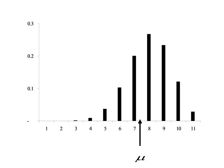
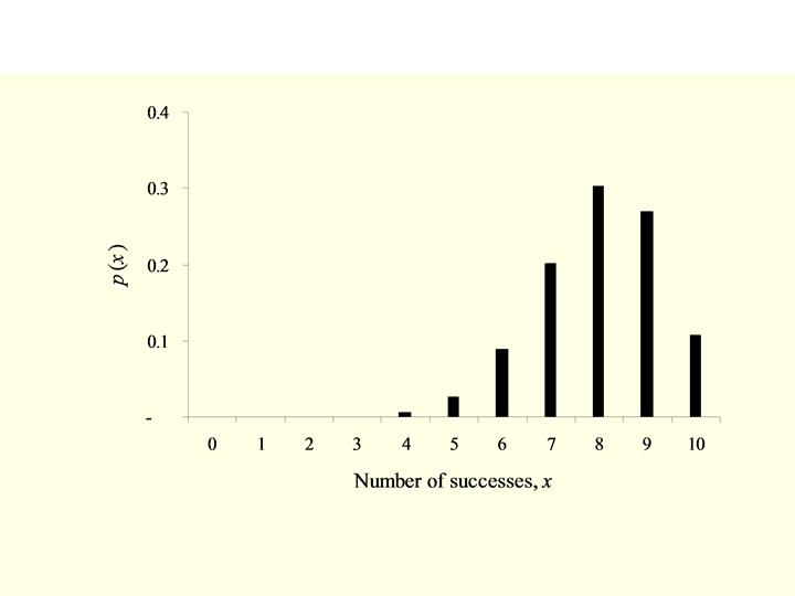
Binomial distribution n = 20, p = 0. 70 Approximating Normal distribution Binomial distribution

Normal Approximation to the Binomial distribution • X has a Binomial distribution with parameters n and p • Y has a Normal distribution
![Approximating Normal distribution P[X = a] Binomial distribution](http://slidetodoc.com/presentation_image_h/279db538cba067b72a97dade9e9a9eee/image-139.jpg "Approximating Normal distribution P[X = a] Binomial distribution")
Approximating Normal distribution P[X = a] Binomial distribution
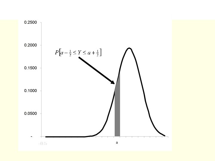
![P[X = a]](http://slidetodoc.com/presentation_image_h/279db538cba067b72a97dade9e9a9eee/image-141.jpg "P[X = a]")
P[X = a]

Example • X has a Binomial distribution with parameters n = 20 and p = 0. 70

Using the Normal approximation to the Binomial distribution Where Y has a Normal distribution with:

Hence = 0. 4052 - 0. 2327 = 0. 1725 Compare with 0. 1643

Normal Approximation to the Binomial distribution • X has a Binomial distribution with parameters n and p • Y has a Normal distribution
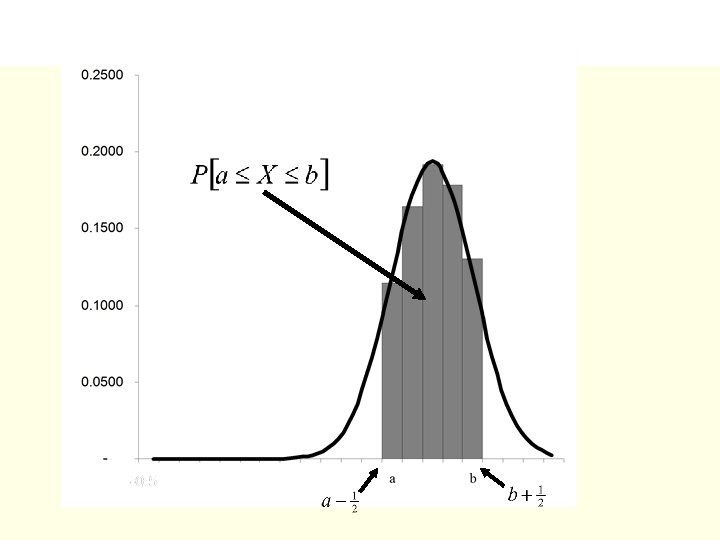


Example • X has a Binomial distribution with parameters n = 20 and p = 0. 70

Using the Normal approximation to the Binomial distribution Where Y has a Normal distribution with:

Hence = 0. 5948 - 0. 0436 = 0. 5512 Compare with 0. 5357

Comment: • The accuracy of the normal appoximation to the binomial increases with increasing values of n

Normal Approximation to the Binomial distribution • X has a Binomial distribution with parameters n and p • Y has a Normal distribution

Example • The success rate for an Eye operation is 85% • The operation is performed n = 2000 times Find 1. The number of successful operations is between 1650 and 1750. 2. The number of successful operations is at most 1800.

Solution • X has a Binomial distribution with parameters n = 2000 and p = 0. 85 where Y has a Normal distribution with:

= 0. 9004 - 0. 0436 = 0. 8008

Solution – part 2. = 1. 000

Next topic: Sampling Theory
- Slides: 157