Probability Rules Statistics 15 Definitions When two events

Probability Rules! Statistics 15

Definitions

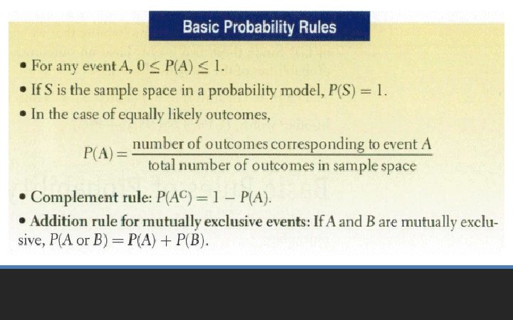
• When two events A and B are disjoint, we can use the addition rule for disjoint events from Chapter 14: P(A B) = P(A) + P(B) • However, when our events are not disjoint, this earlier addition rule will double count the probability of both A and B occurring. Thus, we need the General Addition Rule. • Let’s look at a picture… The General Addition Rule

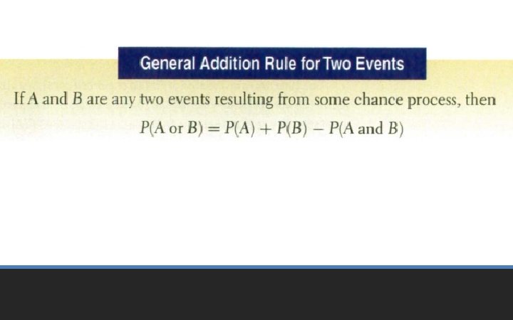
• General Addition Rule: – For any two events A and B, P(A B) = P(A) + P(B) – P(A B) • The following Venn diagram shows a situation in which we would use the general addition rule: The General Addition Rule

Example

• Back in Chapter 3, we looked at contingency tables and talked about conditional distributions. • When we want the probability of an event from a conditional distribution, we write P(B|A) and pronounce it “the probability of B given A. ” • A probability that takes into account a given condition is called a conditional probability. It Depends…

• To find the probability of the event B given the event A, we restrict our attention to the outcomes in A. We then find the fraction of those outcomes B that also occurred. • Note: P(A) cannot equal 0, since we know that A has occurred. It Depends…

• When two events A and B are independent, we can use the multiplication rule for independent events from Chapter 14: P(A B) = P(A) x P(B) • However, when our events are not independent, this earlier multiplication rule does not work. Thus, we need the General Multiplication Rule. The General Multiplication Rule

• We encountered the general multiplication rule in the form of conditional probability. • Rearranging the equation in the definition for conditional probability, we get the General Multiplication Rule: – For any two events A and B, P(A B) = P(A) P(B|A) or P(A B) = P(B) P(A|B) The General Multiplication Rule

• Independence of two events means that the outcome of one event does not influence the probability of the other. • With our new notation for conditional probabilities, we can now formalize this definition: – Events A and B are independent whenever P(B|A) = P(B). (Equivalently, events A and B are independent whenever P(A|B) = P(A). ) Independence

Disjoint

• Disjoint events cannot be independent! Well, why not? – Since we know that disjoint events have no outcomes in common, knowing that one occurred means the other didn’t. – Thus, the probability of the second occurring changed based on our knowledge that the first occurred. – It follows, then, that the two events are not independent. • A common error is to treat disjoint events as if they were independent, and apply the Multiplication Rule for independent events—don’t make that mistake. Independent ≠ Disjoint

• It’s much easier to think about independent events than to deal with conditional probabilities. – It seems that most people’s natural intuition for probabilities breaks down when it comes to conditional probabilities. • Don’t fall into this trap: whenever you see probabilities multiplied together, stop and ask whether you think they are really independent. Depending on Independence

• Sampling without replacement means that once one individual is drawn it doesn’t go back into the pool. – We often sample without replacement, which doesn’t matter too much when we are dealing with a large population. – However, when drawing from a small population, we need to take note and adjust probabilities accordingly. • Drawing without replacement is just another instance of working with conditional probabilities. Drawing Without Replacement

• A tree diagram helps us think through conditional probabilities by showing sequences of events as paths that look like branches of a tree. • Making a tree diagram for situations with conditional probabilities is consistent with our “make a picture” mantra. Tree Diagrams

• This is an example of a tree diagram and shows how we multiply the probabilities of the branches together. • All the final outcomes are disjoint and must add up to one. • We can add the final probabilities to find probabilities of compound events. Tree Diagrams

From a standard deck of cards. One card is drawn. What is the probability it is an ace or red? Example

From a standard deck of cards. Two cards are drawn without replacement. What is the probability they are both aces? Extend to the probability of getting 5 hearts in a row. Example

From a standard deck of cards. I draw one card and look at it. I tell you it is red. What is the probability it is a heart? And what is the probability it is red, given that it is a heart? Example

• Reversing the conditioning of two events is rarely intuitive. • Suppose we want to know P(A|B), and we know only P(A), P(B), and P(B|A). • We also know P(A B), since P(A B) = P(A) x P(B|A) • From this information, we can find P(A|B): Reversing the Conditioning

Example

• When we reverse the probability from the conditional probability that you’re originally given, you are actually using Bayes’s Rule

• Don’t use a simple probability rule where a general rule is appropriate: – Don’t assume that two events are independent or disjoint without checking that they are. • Don’t find probabilities for samples drawn without replacement as if they had been drawn with replacement. • Don’t reverse conditioning naively. • Don’t confuse “disjoint” with “independent. ” What Can Go Wrong?

• The probability rules from Chapter 14 only work in special cases—when events are disjoint or independent. • We now know the General Addition Rule and General Multiplication Rule. • We also know about conditional probabilities and that reversing the conditioning can give surprising results. What have we learned?

• Venn diagrams, tables, and tree diagrams help organize our thinking about probabilities. • We now know more about independence—a sound understanding of independence will be important throughout the rest of this course. What have we learned?

• Pages 363 – 366 • 3, 6, 8, 9, 11, 14, 22, 25, 29, 34, 40, 42 Homework