Probability Review The state of the world is

Probability: Review • The state of the world is described using random variables • Probabilities are defined over events – Sets of world states characterized by propositions about random variables – E. g. , D 1, D 2: rolls of two dice • P(D 1 > 2) • P(D 1 + D 2 = 11) – W is the state of the weather • P(W = “rainy” W = “sunny”)

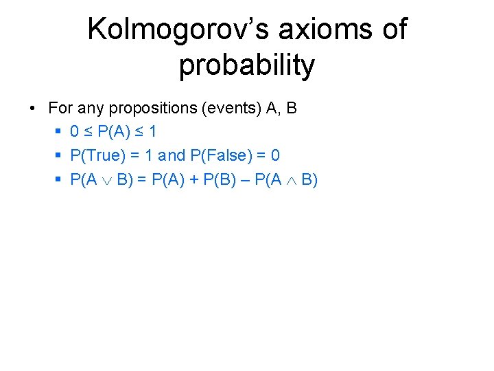
Kolmogorov’s axioms of probability • For any propositions (events) A, B § 0 ≤ P(A) ≤ 1 § P(True) = 1 and P(False) = 0 § P(A B) = P(A) + P(B) – P(A B)

Joint probability distributions • A joint distribution is an assignment of probabilities to every possible atomic event P(Cavity, Toothache) Cavity = false Toothache = false 0. 8 Cavity = false Toothache = true 0. 1 Cavity = true Toothache = false 0. 05 Cavity = true Toothache = true 0. 05

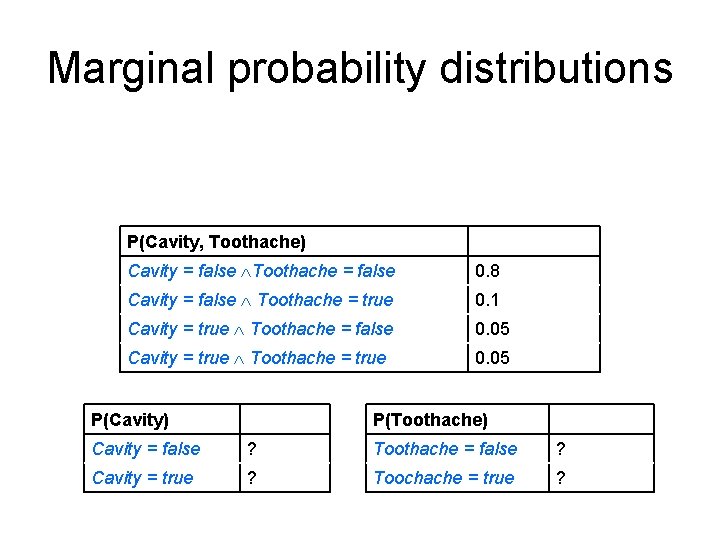
Marginal probability distributions P(Cavity, Toothache) Cavity = false Toothache = false 0. 8 Cavity = false Toothache = true 0. 1 Cavity = true Toothache = false 0. 05 Cavity = true Toothache = true 0. 05 P(Cavity) P(Toothache) Cavity = false ? Toothache = false ? Cavity = true ? Toochache = true ?

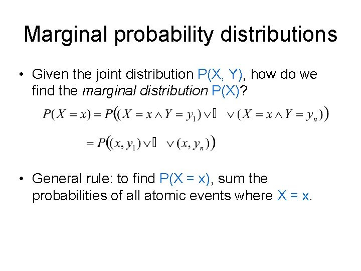
Marginal probability distributions • Given the joint distribution P(X, Y), how do we find the marginal distribution P(X)? • General rule: to find P(X = x), sum the probabilities of all atomic events where X = x.

Conditional probability

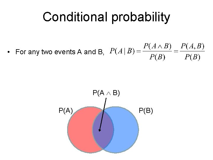
Conditional probability • For any two events A and B, P(A B) P(A) P(B)

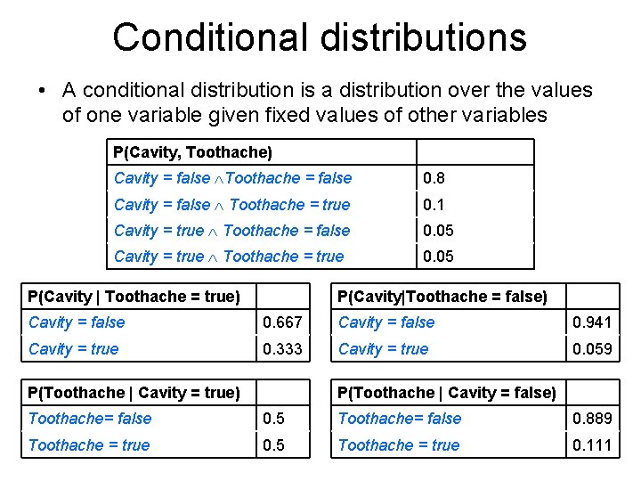
Conditional distributions • A conditional distribution is a distribution over the values of one variable given fixed values of other variables P(Cavity, Toothache) Cavity = false Toothache = false 0. 8 Cavity = false Toothache = true 0. 1 Cavity = true Toothache = false 0. 05 Cavity = true Toothache = true 0. 05 P(Cavity | Toothache = true) P(Cavity|Toothache = false) Cavity = false 0. 667 Cavity = false 0. 941 Cavity = true 0. 333 Cavity = true 0. 059 P(Toothache | Cavity = true) P(Toothache | Cavity = false) Toothache= false 0. 5 Toothache= false 0. 889 Toothache = true 0. 5 Toothache = true 0. 111

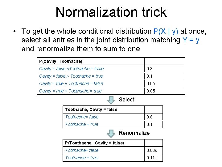
Normalization trick • To get the whole conditional distribution P(X | y) at once, select all entries in the joint distribution matching Y = y and renormalize them to sum to one P(Cavity, Toothache) Cavity = false Toothache = false 0. 8 Cavity = false Toothache = true 0. 1 Cavity = true Toothache = false 0. 05 Cavity = true Toothache = true 0. 05 Select Toothache, Cavity = false Toothache= false 0. 8 Toothache = true 0. 1 Renormalize P(Toothache | Cavity = false) Toothache= false 0. 889 Toothache = true 0. 111

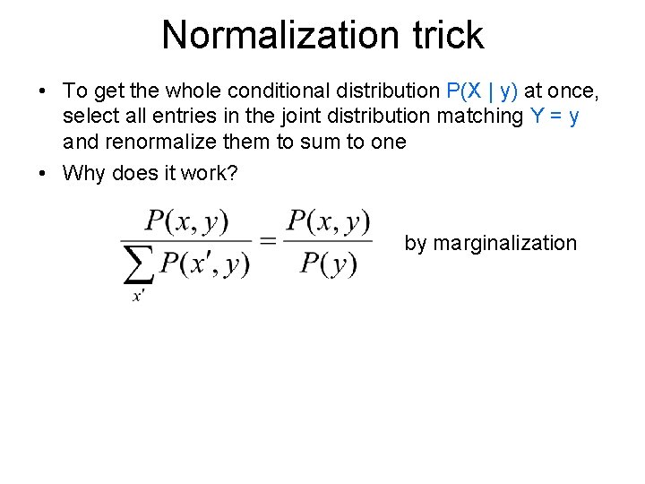
Normalization trick • To get the whole conditional distribution P(X | y) at once, select all entries in the joint distribution matching Y = y and renormalize them to sum to one • Why does it work? by marginalization

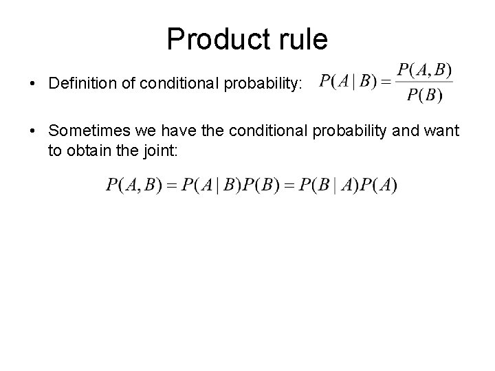
Product rule • Definition of conditional probability: • Sometimes we have the conditional probability and want to obtain the joint:

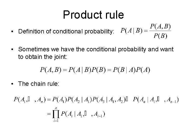
Product rule • Definition of conditional probability: • Sometimes we have the conditional probability and want to obtain the joint: • The chain rule:

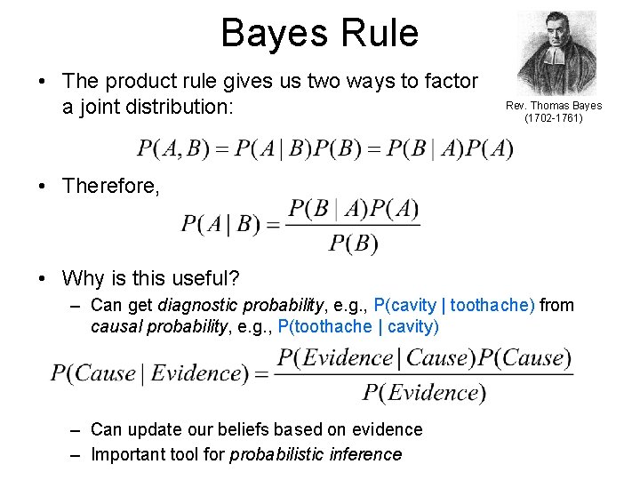
Bayes Rule • The product rule gives us two ways to factor a joint distribution: Rev. Thomas Bayes (1702 -1761) • Therefore, • Why is this useful? – Can get diagnostic probability, e. g. , P(cavity | toothache) from causal probability, e. g. , P(toothache | cavity) – Can update our beliefs based on evidence – Important tool for probabilistic inference

Independence • Two events A and B are independent if and only if P(A, B) = P(A) P(B) – In other words, P(A | B) = P(A) and P(B | A) = P(B) – This is an important simplifying assumption for modeling, e. g. , Toothache and Weather can be assumed to be independent • Are two mutually exclusive events independent? – No, but for mutually exclusive events we have P(A B) = P(A) + P(B) • Conditional independence: A and B are conditionally independent given C iff P(A, B | C) = P(A | C) P(B | C)

Conditional independence: Example • Toothache: boolean variable indicating whether the patient has a toothache • Cavity: boolean variable indicating whether the patient has a cavity • Catch: whether the dentist’s probe catches in the cavity • If the patient has a cavity, the probability that the probe catches in it doesn't depend on whether he/she has a toothache P(Catch | Toothache, Cavity) = P(Catch | Cavity) • Therefore, Catch is conditionally independent of Toothache given Cavity • Likewise, Toothache is conditionally independent of Catch given Cavity P(Toothache | Catch, Cavity) = P(Toothache | Cavity) • Equivalent statement: P(Toothache, Catch | Cavity) = P(Toothache | Cavity) P(Catch | Cavity)

Conditional independence: Example • How many numbers do we need to represent the joint probability table P(Toothache, Cavity, Catch)? 23 – 1 = 7 independent entries • Write out the joint distribution using chain rule: P(Toothache, Catch, Cavity) = P(Cavity) P(Catch | Cavity) P(Toothache | Cavity) • How many numbers do we need to represent these distributions? 1 + 2 = 5 independent numbers • In most cases, the use of conditional independence reduces the size of the representation of the joint distribution from exponential in n to linear in n

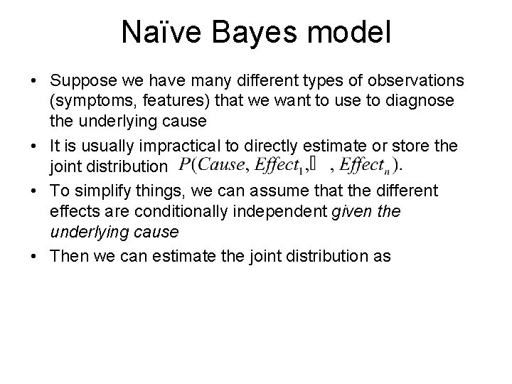
Naïve Bayes model • Suppose we have many different types of observations (symptoms, features) that we want to use to diagnose the underlying cause • It is usually impractical to directly estimate or store the joint distribution • To simplify things, we can assume that the different effects are conditionally independent given the underlying cause • Then we can estimate the joint distribution as

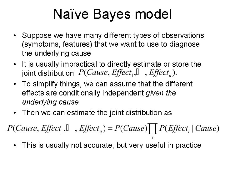
Naïve Bayes model • Suppose we have many different types of observations (symptoms, features) that we want to use to diagnose the underlying cause • It is usually impractical to directly estimate or store the joint distribution • To simplify things, we can assume that the different effects are conditionally independent given the underlying cause • Then we can estimate the joint distribution as • This is usually not accurate, but very useful in practice

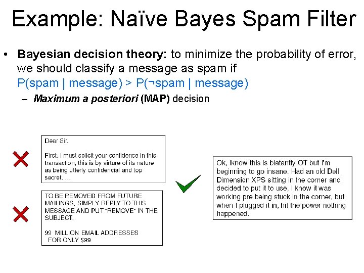
Example: Naïve Bayes Spam Filter • Bayesian decision theory: to minimize the probability of error, we should classify a message as spam if P(spam | message) > P(¬spam | message) – Maximum a posteriori (MAP) decision

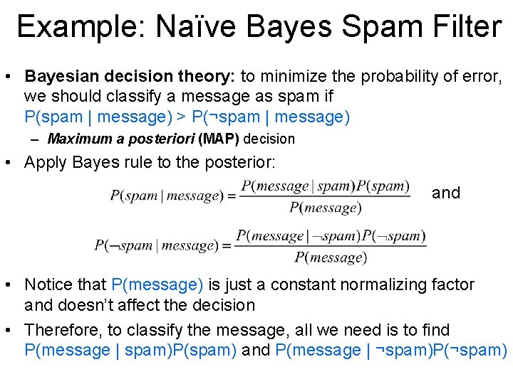
Example: Naïve Bayes Spam Filter • Bayesian decision theory: to minimize the probability of error, we should classify a message as spam if P(spam | message) > P(¬spam | message) – Maximum a posteriori (MAP) decision • Apply Bayes rule to the posterior: and • Notice that P(message) is just a constant normalizing factor and doesn’t affect the decision • Therefore, to classify the message, all we need is to find P(message | spam)P(spam) and P(message | ¬spam)P(¬spam)

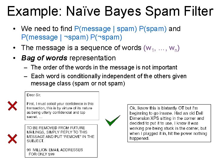
Example: Naïve Bayes Spam Filter • We need to find P(message | spam) P(spam) and P(message | ¬spam) P(¬spam) • The message is a sequence of words (w 1, …, wn) • Bag of words representation – The order of the words in the message is not important – Each word is conditionally independent of the others given message class (spam or not spam)

Bag of words illustration US Presidential Speeches Tag Cloud http: //chir. ag/projects/preztags/

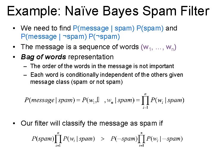
Example: Naïve Bayes Spam Filter • We need to find P(message | spam) P(spam) and P(message | ¬spam) P(¬spam) • The message is a sequence of words (w 1, …, wn) • Bag of words representation – The order of the words in the message is not important – Each word is conditionally independent of the others given message class (spam or not spam) • Our filter will classify the message as spam if

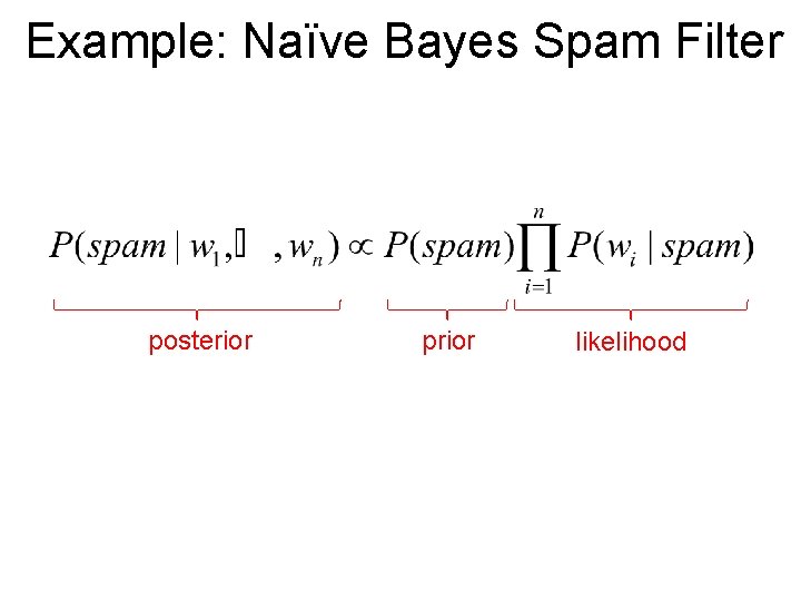
Example: Naïve Bayes Spam Filter posterior prior likelihood

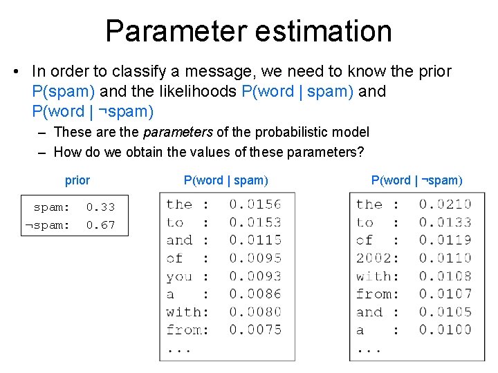
Parameter estimation • In order to classify a message, we need to know the prior P(spam) and the likelihoods P(word | spam) and P(word | ¬spam) – These are the parameters of the probabilistic model – How do we obtain the values of these parameters? prior spam: ¬spam: 0. 33 0. 67 P(word | spam) P(word | ¬spam)

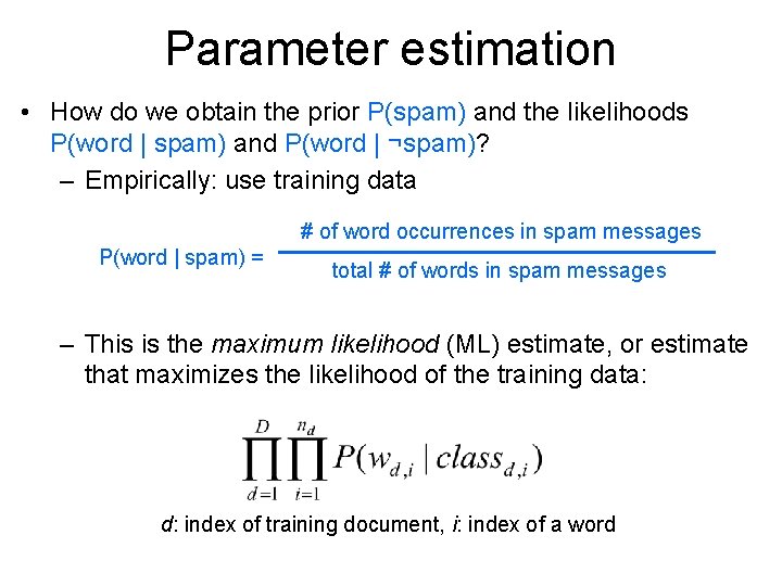
Parameter estimation • How do we obtain the prior P(spam) and the likelihoods P(word | spam) and P(word | ¬spam)? – Empirically: use training data # of word occurrences in spam messages P(word | spam) = total # of words in spam messages – This is the maximum likelihood (ML) estimate, or estimate that maximizes the likelihood of the training data: d: index of training document, i: index of a word