Probability in Robotics Trends in Robotics Research Classical

Probability in Robotics

Trends in Robotics Research Classical Robotics (mid-70’s) • exact models • no sensing necessary Reactive Paradigm (mid-80’s) • no models • relies heavily on good sensing Hybrids (since 90’s) • model-based at higher levels • reactive at lower levels Probabilistic Robotics (since mid-90’s) • seamless integration of models and sensing • inaccurate models, inaccurate sensors

Advantages of Probabilistic Paradigm • Can accommodate inaccurate models • Can accommodate imperfect sensors • Robust in real-world applications • Best known approach to many hard robotics problems • Pays Tribute to Inherent Uncertainty Know your own ignorance • Scalability • No need for “perfect” world model Relieves programmers

Limitations of Probability • Computationally inefficient – Consider entire probability densities • Approximation – Representing continuous probability distributions.

Uncertainty Representation

Five Sources of Uncertainty Approximate Computation Environment Dynamics Random Action Effects Inaccurate Models Sensor Limitations

Why Probabilities Real environments imply uncertainty in accuracy of robot actions sensor measurements Robot accuracy and correct models are vital for successful operations All available data must be used A lot of data is available in the form of probabilities 7

What Probabilities Sensor parameters Sensor accuracy Robot wheels slipping Motor resolution limited Wheel precision limited Performance alternates on temperature, etc. based 8

Reasons for Motion Errors ideal case bump and many more … different wheel diameters carpet 9

What Probabilities These inaccuracies can be measured and modelled with random distributions Single reading of a sensor contains more information given the prior probability distribution of sensor behavior than its actual value Robot cannot afford throwing away this additional information! 10

What Probabilities More advanced concepts: Robot position and orientation (robot pose) Map of the environment Planning and control Action selection Reasoning. . . 11

Probabilistic Robotics • Falls in between model-based and behaviorbased techniques – There are models, and sensor measurements, but they are assumed to be incomplete and insufficient for control – Statistics provides the mathematical glue to integrate models and sensor measurements • Basic Mathematics – Probabilities – Bayes rule – Bayes filters 12

Nature of Sensor Data Odometry Data Range Data

Sensor inaccuracy Environmental Uncertainty

How do we Solve Localization Uncertainty? • Represent beliefs as a probability density • Markov assumption Pose distribution at time t conditioned on: pose dist. at time t-1 movement at time t-1 sensor readings at time t • Discretize the density by sampling More on this later….

Probabilistic Action model At every time step t: UPDATE each sample’s new location based on movement RESAMPLE the pose distribution based on sensor readings p(st|at-1, st-1) st-1 at-1 • Continuous probability density Bel(st) after moving 40 m (left figure) and 80 m (right figure). Darker area has higher probablity.

Globalization Localization without knowledge of start location n

Probabilistic Robotics: Basic Idea Key idea: Explicit representation of uncertainty using probability theory • Perception = state estimation • Action = utility optimization

Advantages and Pitfalls • • Can accommodate inaccurate models Can accommodate imperfect sensors Robust in real-world applications Best known approach to many hard robotics problems Computationally demanding False assumptions Approximate

Axioms of Probability Theory Pr(A) denotes probability that proposition A is true.

A Closer Look at Axiom 3 B

Using the Axioms

Discrete Random Variables • X denotes a random variable. • X can take on a finite number of values in {x 1, x 2, …, xn}. • P(X=xi), or P(xi), is the probability that the random variable X takes on value xi. • P( ) is called probability mass function. • E. g.

Continuous Random Variables • X takes on values in the continuum. • p(X=x), or p(x), is a probability density function. • E. g. p(x) x

Joint and Conditional Probability • P(X=x and Y=y) = P(x, y) • If X and Y are independent then P(x, y) = P(x) P(y) • P(x | y) is the probability of x given y P(x | y) = P(x, y) / P(y) P(x, y) = P(x | y) P(y) • If X and Y are independent then P(x | y) = P(x)

Law of Total Probability Discrete case Continuous case

Thomas Bayes (1702 -1761) Mathematician who first used probability inductively and established a mathematical basis for probability inference

Bayes Formula

Normalization

Conditioning • Total probability: • Bayes rule and background knowledge:

Simple Example of State Estimation • Suppose a robot obtains measurement z • What is P(open|z)?

Causal vs. Diagnostic Reasoning • • P(open|z) is diagnostic. P(z|open) is causal. Often causal knowledge is easier to obtain. Bayes rule allows us to use causal knowledge to calculate diagnostic: count frequencies!

Example • P(z|open) = 0. 6 • P(open) = P( open) = 0. 5 P(z| open) = 0. 3 • z raises the probability that the door is open.

Combining Evidence • Suppose our robot obtains another observation z 2. • How can we integrate this new information? • More generally, how can we estimate P(x| z 1. . . zn )?

Recursive Bayesian Updating Markov assumption: zn is independent of z 1, . . . , zn-1 if we know x.

Example: Second Measurement • P(z 2|open) = 0. 5 P(z 2| open) = 0. 6 • P(open|z 1)=2/3 • z 2 lowers the probability that the door is open.

Localization, Where am I? • Localization base on external sensors, beacons or landmarks • Probabilistic Map Based Localization Perception • Odometry, Dead Reckoning

Localization Methods • Mathematical Background, Bayes Filter • Markov Localization: – Central idea: represent the robot’s belief by a probability distribution over possible positions, and uses Bayes’ rule and convolution to update the belief whenever the robot senses or moves – Markov Assumption: past and future data are independent if one knows the current state • Kalman Filtering – Central idea: posing localization problem as a sensor fusion problem – Assumption: gaussian distribution function • Particle Filtering – Central idea: Sample-based, nonparametric Filter – Monte-Carlo method • SLAM (simultaneous localization and mapping) • Multi-robot localization 39

Markov Localization • Applying probability theory to robot localization • Markov localization uses an explicit, discrete representation for the probability of all position in the state space. • This is usually done by representing the environment by a grid or a topological graph with a finite number of possible states (positions). • During each update, the probability for each state (element) of the entire space is updated. 40

Markov Localization Example • Assume the robot position is one- dimensional The robot is placed somewhere in the environment but it is not told its location The robot queries its sensors and finds out it is next to a door 41

Markov Localization Example The robot moves one meter forward. To account for inherent noise in robot motion the new belief is smoother The robot queries its sensors and again it finds itself next to a door 42

Markov Process • Markov Property: The state of the system at time t+1 depends only on the state of the system at time t X 1 X 2 X 4 X 3 X 5 • Stationary Assumption: Transition probabilities are independent of time (t) 43

Markov Process Simple Example Bumper Sensor: • hits wall 40% will hit in next position 60% will not hit next position • not hit wall 20% will hit in next position 80% will not hit next position Stochastic FSM: 0. 6 0. 4 hit 0. 8 no hit 0. 2 44

Markov Process Simple Example Bumper Sensor: • hits wall 40% will hit in next position 60% will not hit next position • not hit wall 20% will hit in next position 80% will not hit next position The transition matrix: • Stochastic matrix: Rows sum up to 1 • Double stochastic matrix: Rows and columns sum up to 1 45

Markov Process obstacle vs. No-obstacle Example • Given that a robot’s last sonar reading was Obstacle, there is a 90% chance that its next reading will also be Obstacle. • If a robot’s last sonar reading was No-obstacle, there is an 80% chance that its next reading will also be No-obstacle. transition matrix: Obst. No-obst. 0. 1 0. 9 Obst. No-obst 0. 2 No-obst. 46 0. 8

Markov Process obstacle vs. No-obstacle Example Given that a robot is currently reading No-obstacle, what is the probability that it will read obstacle two readings from now? Pr[ no-obstacle ? obstacle ] = Pr[ no-obst ] + Pr[ no-obst ] = 0. 2 * 0. 9 no-obst ? + 0. 8 ? obst 47 * 0. 2 = 0. 34

Markov Process obstacle vs. No-obstacle Example Given that a robot is currently reading obstacle, what is the probability that it will read no-obstacle three readings from now? 48

Markov Process obstacle vs. No-obstacle Example • Assume each sensor makes one reading per second • Suppose 60% of all sensors now read obstacle, and 40% read no-obstacle • What fraction of sensors will be reading obstacle three seconds from now? Pr[X 3=obs] = 0. 6 * 0. 781 + 0. 4 * 0. 438 = 0. 6438 Qi - the distribution in second i Q 0=(0. 6, 0. 4) - initial distribution Q 3= Q 0 * P 3 =(0. 6438, 0. 3562) 49

Markov Process obstacle vs. No-obstacle Example Simulation: Pr[Xi = obst] 2/3 stationary distribution 0. 1 0. 9 obst 0. 8 No-obst 0. 2 second - 50 i

Actions • Often the world is dynamic since – actions carried out by the robot, – actions carried out by other agents, – or just the time passing by change the world. • How can we incorporate such actions?

Typical Actions • The robot turns its wheels to move • The robot uses its manipulator to grasp an object • Actions are never carried out with absolute certainty. • In contrast to measurements, actions generally increase the uncertainty.

Modeling Actions • To incorporate the outcome of an action u into the current “belief”, we use the conditional pdf P(x|u, x’) • This term specifies the pdf that executing u changes the state from x’ to x.

Terminology • Robot State (or pose): xt =[ x, y, θ] – Position and heading – x 1: t = {x 1, …, xt} • Robot Controls: ut – Robot motion and manipulation – u 1: t = {u 1, . . . , ut} • Sensor Measurements: zt – Range scans, images, etc. – z 1: t = {z 1, . . . , zt} • Landmark or Map: – Landmarks or Map

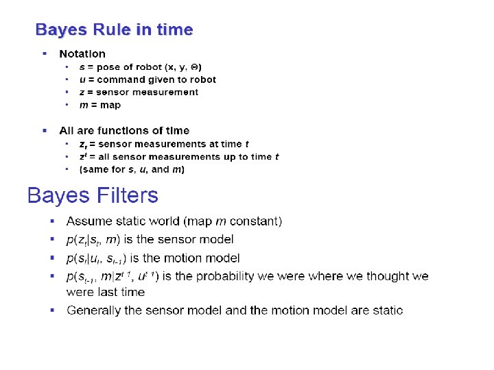
Terminology • Observation model: or – The probability of a measurement zt given that the robot is at position xt and map m. • Motion Model: – The posterior probability that action ut carries the robot from xt-1 to xt.

Terminology • Belief: bel(x t ) – Posterior probability – Conditioned on available data – • Prediction: bel(x t ) – Estimate before measurement data –

Example: Closing the door

State Transitions P(x|u, x’) for u = “close door”: If the door is open, the action “close door” succeeds in 90% of all cases.

Integrating the Outcome of Actions Continuous case: Discrete case:

Example: The Resulting Belief

Robot Environment Interaction State transition probability measurement probability

Bayes Filters: Framework Given: Stream of observations z and action data u: Sensor model P(z|x). Action model P(x|u, x’). Prior probability of the system state P(x). Wanted: Estimate of the state X of a dynamical system. The posterior of the state is also called Belief:

Markov Assumption Underlying Assumptions Static world Independent noise Perfect model, no approximation errors

Bayes Filters: Framework • Given: – Stream of observations z and action data u: measurement probability – Sensor model P(z|x). State transition probability – Action model P(x|u, x’). – Prior probability of the system state P(x). • Wanted: – Estimate of the state X of a dynamical system. – The posterior of the state is called Belief: 64

Bayes Filters: The Algorithm • Algorithm Bayes_filter ( • for all • • • endfor return do ) Action model Sensor model 65

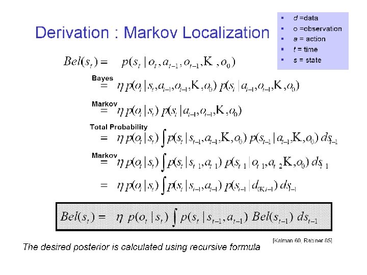
Bayes Filters z = observation u = action x = state Bayes Markov Total prob. Markov Sensor model Action model recursion 66

Bayes Filter Algorithm • • Algorithm Bayes_filter( Bel(x), d ): 0 • • • If d is a perceptual data item z then For all x do • • • Else if d is an action data item u then For all x do • Return Bel’(x) For all x do

Bayes Filters are Familiar! Kalman filters (a recursive Bayesian filter for multivariate normal distributions) Particle filters (a sequential Monte Carlo (SMC) based technique, which models the PDF using a set of discrete points) Hidden Markov models (Markov process with unknown parameters) Dynamic Bayesian networks Partially Observable Markov Decision Processes (POMDPs)

In summary……. Bayes rule allows us to compute probabilities that are hard to assess otherwise Under the Markov assumption, recursive Bayesian updating can be used to efficiently combine evidence Bayes filters are a probabilistic tool for estimating the state of dynamic systems.

How all of this relates to Sensors and navigation? Sensor fusion

Basic statistics – Statistical representation – Stochastic variable Travel time, X = 5 hours ± 1 hour X can have many different values Continous – The variable can have any value within the bounds Discrete – The variable can have specific (discrete) values

Basic statistics – Statistical representation – Stochastic variable Another way of describing the stochastic variable, i. e. by another form of bounds Probability distribution In 68%: x 11 < X < x 12 In 95%: x 21 < X < x 22 In 99%: x 31 < X < x 32 In 100%: - < X < The value to expect is the mean value => Expected value How much X varies from its expected value => Variance

Expected value and Variance The standard deviation X is the square root of the variance

Gaussian (Normal) distribution By far the mostly used probability distribution because of its nice statistical and mathematical properties What does it means if a specification tells that a sensor measures a distance [mm] and has an error that is normally distributed with zero mean and = 100 mm? Normal distribution: ~68. 3% ~95% ~99% etc.

Estimate of the expected value and the variance from observations

Linear combinations (1) X 2 ~ N(m 2, σ2) X 1 ~ N(m 1, σ1) Y ~ N(m 1 + m 2, sqrt(σ1 +σ2)) Since linear combination of Gaussian variables is another Gaussian variable, Y remains Gaussian if the s. v. are combined linearly!

Linear combinations (2) We measure a distance by a device that have normally distributed errors, Do we win something of making a lot of measurements and use the average value instead? What will the expected value of Y be? What will the variance (and standard deviation) of Y be? If you are using a sensor that gives a large error, how would you best use it?

Linear combinations (3) di is the mean value and d ~ N(0, σd) αi is the mean value and α ~ N(0, σα) With d and α uncorrelated => V[ d, α] = 0 (co-variance is zero)

Linear combinations (4) D = {The total distance} is calculated as before as this is only the sum of all d’s The expected value and the variance become:

Linear combinations (5) = {The heading angle} is calculated as before as this is only the sum of all ’s, i. e. as the sum of all changes in heading The expected value and the variance become: What if we want to predict X and Y from our measured d’s and ’s?

Non-linear combinations (1) X(N) is the previous value of X plus the latest movement (in the X direction) The estimate of X(N) becomes: This equation is non-linear as it contains the term: and for X(N) to become Gaussian distributed, this equation must be replaced with a linear approximation around. To do this we can use the Taylor expansion of the first order. By this approximation we also assume that the error is rather small! With perfectly known N-1 and N-1 the equation would have been linear!

Non-linear combinations (2) Use a first order Taylor expansion and linearize X(N) around . This equation is linear as all error terms are multiplied by constants and we can calculate the expected value and the variance as we did before.

Non-linear combinations (3) The variance becomes (calculated exactly as before): Two really important things should be noticed, first the linearization only affects the calculation of the variance and second (which is even more important) is that the above equation is the partial derivatives of: with respect to our uncertain parameters squared multiplied with their variance!

Non-linear combinations (4) This result is very good => an easy way of calculating the variance => the law of error propagation The partial derivatives of become:

Non-linear combinations (5) The plot shows the variance of X for the time step 1, …, 20 and as can be noticed the variance (or standard deviation) is constantly increasing. d = 1/10 = 5/360

The Error Propagation Law

The Error Propagation Law

The Error Propagation Law

Multidimensional Gaussian distributions MGD (1) The Gaussian distribution can easily be extended for several dimensions by: replacing the variance ( ) by a co-variance matrix ( ) and the scalars (x and m. X) by column vectors. The CVM describes (consists of): 1) the variances of the individual dimensions => diagonal elements 2) the co-variances between the different dimensions => off-diagonal elements ! Symmetric ! Positive definite

A 1 -d Gaussian distribution is given by: An n-d Gaussian distribution is given by:

MGD (2) Eigenvalues => standard deviations Eigenvectors => rotation of the ellipses

MGD (3) The co-variance between two stochastic variables is calculated as: Which for a discrete variable becomes: And for a continuous variable becomes:

MGD (4) - Non-linear combinations The state variables (x, y, ) at time k+1 become:

MGD (5) - Non-linear combinations We know that to calculate the variance (or co-variance) at time step k+1 we must linearize Z(k+1) by e. g. a Taylor expansion - but we also know that this is done by the law of error propagation, which for matrices becomes: With f. X and f. U are the Jacobian matrices (w. r. t. our uncertain variables) of the state transition matrix.

MGD (6) - Non-linear combinations The uncertainty ellipses for X and Y (for time step 1. . 20) is shown in the figure.

Circular Error Problem If we have a map: We can localize! NOT THAT SIMPLE! If we can localize: We can make a map!

Expectation-Maximization (EM) Algorithm • Initialize: Make random guess for lines • Repeat: – Find the line closest to each point and group into two sets. (Expectation Step) – Find the best-fit lines to the two sets (Maximization Step) – Iterate until convergence The algorithm is guaranteed to converge to some local optima

Example:

Example:

Example:

Example:

Example: Converged!

Probabilistic Mapping Maximum Likelihood Estimation • E-Step: Use current best map and data to find belief probabilities • M-step: Compute the most likely map based on the probabilities computed in the E-step. • Alternate steps to get better map and localization estimates Convergence is guaranteed as before.

The E-Step • P(st|d, m) = P(st |o 1, a 1… ot, m). P(st |at…o. T, m) t Bel(st) Markov Localization t Analogous to but computed backward in time

The M-Step • • Updates occupancy grid P(mxy=l | d) = # of times l was observed at <x, y> # of times something was obs. at <x, y>

Probabilistic Mapping • Addresses the Simultaneous Mapping and Localization problem (SLAM) • Robust • Hacks for easing computational and processing burden – Caching – Selective computation – Selective memorization

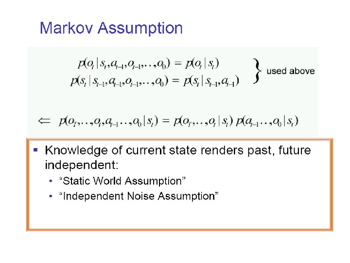
Markov Assumption Future is Independent of Past Given Current State “Assume Static World”

Probabilistic Model Action Data Observation Data

Derivation : Markov Localization Bayes Markov Total Probability Markov

Mobile Robot Localization • Proprioceptive Sensors: (Encoders, IMU) - Odometry, Dead reckoning • Exteroceptive Sensors: (Laser, Camera) - Global, Local Correlation Scan-Matching Scan 1 Scan 2 Initial Guess Point Correspondence Scan-Matching Iterate Displacement Estimate • Correlate range measurements to estimate displacement • Can improve (or even replace) odometry – Roumeliotis TAI-14 • Previous Work - Vision community and Lu & Milios [97]

Weighted Approach Explicit models of uncertainty & noise sources for each scan point: Correspondence Errors • Sensor noise & errors • Range noise • Angular uncertainty • Bias • Point correspondence uncertainty Combined Uncertanties Improvement vs. unweighted method: x 500 1 m • More accurate displacement estimate • More realistic covariance estimate • Increased robustness to initial conditions • Improved convergence

Weighted Formulation Goal: Estimate displacement (pij , fij ) Measured range data from poses i and j sensor noise bias true range Error between kth scan point pair = rotation of fij Noise Error Bias Error Correspondence Error

Covariance of Error Estimate Covariance of error between kth scan point pair = sq 1) Sensor Noise Lik Pose i 2) Sensor Bias neglect for now Correspondence Bias Sensor Noise sl

3) Correspondence Error = cijk Estimate bounds of cijk from the geometry of the boundary and robot poses Max error • Assume uniform distribution where

Finding incidence angles ik and jk Hough Transform -Fits lines to range data -Local incidence angle estimated from line tangent and scan angle -Common technique in vision community (Duda & Hart [72]) -Can be extended to fit simple curves ik Scan Points Fit Lines

Maximum Likelihood Estimation Likelihood of obtaining errors { ijk} given displacement Non-linear Optimization Problem • Position displacement estimate obtained in closed form • Orientation estimate found using 1 -D numerical optimization, or series expansion approximation methods

Experimental Results Weighted vs. Unweighted matching of two poses 512 trials with different initial displacements within : +/- 15 degrees of actual angular displacement +/- 150 mm of actual spatial displacement Initial Displacements Unweighted Estimates Weighted Estimates • Increased robustness to inaccurate initial displacement guesses • Fewer iterations for convergence

Unweighted Weighted

Eight-step, 22 meter path Displacement estimate errors at end of path • Odometry = 950 mm • Unweighted = 490 mm • Weighted = 120 mm More accurate covariance estimate - Improved knowledge of measurement uncertainty - Better fusion with other sensors

Uncertainty From Sensor Noise and Correspondence Error x 500 1 m