Probability Frequentist versus Bayesian and why it matters
Probability Frequentist versus Bayesian and why it matters Roger Barlow Manchester University 11 th February 2008
Outline n n n Different definitions of probability: Frequentist and Bayesian Measurements: definitions usually give the same results Differences in dealing with q q q n n Nongaussian measurements Small number counting Constrained parameters Difficulties for both Conclusions and recommendations Frequentist and Bayesian Probability Roger Barlow 2
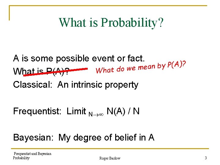
What is Probability? A is some possible event or fact. (A)? P y b n a e m e What do w What is P(A)? Classical: An intrinsic property Frequentist: Limit N N(A) / N Bayesian: My degree of belief in A Frequentist and Bayesian Probability Roger Barlow 3
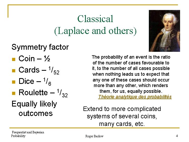
Classical (Laplace and others) Symmetry factor n Coin – ½ n Cards – 1/52 n Dice – 1/6 n Roulette – 1/32 Equally likely outcomes Frequentist and Bayesian Probability The probability of an event is the ratio of the number of cases favourable to it, to the number of all cases possible when nothing leads us to expect that any one of these cases should occur more than any other, which renders them, for us, equally possible. Théorie analytique des probabilités Extend to more complicated systems of several coins, many cards, etc. Roger Barlow 4
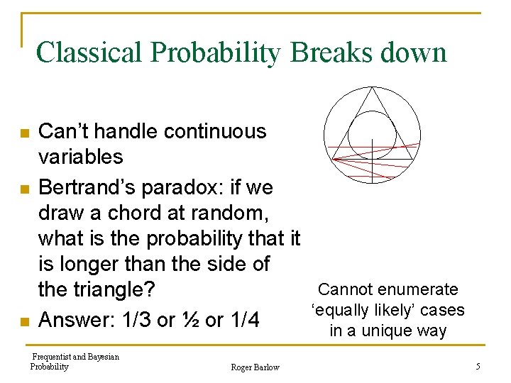
Classical Probability Breaks down n Can’t handle continuous variables Bertrand’s paradox: if we draw a chord at random, what is the probability that it is longer than the side of the triangle? Answer: 1/3 or ½ or 1/4 Frequentist and Bayesian Probability Roger Barlow Cannot enumerate ‘equally likely’ cases in a unique way 5
Frequentist Probability (von Mises, Fisher) A Ensemble of Everything Limit of frequency P(A)= Limit N N(A)/N This was a property of the classical definition, now promoted to become a definition itself P(A) depends not just on A but on the ensemble – which must be specified. This leads to two surprising features Frequentist and Bayesian Probability Roger Barlow 6
Feature 1: There can be many Ensembles Probabilities belong to the event and the ensemble n Insurance company data shows P(death) for 40 year old male clients = 1. 4% (example due to von Mises) n Does this mean a particular 40 year old German has a 98. 6% chance of reaching his 41 st Birthday? n No. He belongs to many ensembles q German insured males q German males q Insured nonsmoking vegetarians q German insured male racing drivers q … Each of these gives a different number. All equally valid. n Frequentist and Bayesian Probability Roger Barlow 7
Feature 2: Unique events have no ensemble Some events are unique. Consider “It will probably rain tomorrow. ” There is only one tomorrow (Tuesday 12 th February). There is NO ensemble. P(rain) is either 0/1 =0 or 1/1 = 1 Strict frequentists cannot say 'It will probably rain tomorrow'. This presents severe social problems. Frequentist and Bayesian Probability Roger Barlow 8
Circumventing the limitation A frequentist can say: “The statement ‘It will rain tomorrow’ has a 70% probability of being true. ” by assembling an ensemble of statements and ascertaining that 70% (say) are true. (E. g. Weather forecasts with a verified track record) Say “It will rain tomorrow” with 70% confidence For unique events, confidence level statements replace probability statements. Frequentist and Bayesian Probability Roger Barlow 9
Bayesian (Subjective) Probability P(A) is a number describing my degree of belief in A 1=certain belief. 0=total disbelief Can be calibrated against simple classical probabilities. P(A)=0. 5 means: I would be indifferent given the choice of betting on A or betting on a coin toss. A can be anything: death, rain, horse races, existence of SUSY… Very adaptable. But no guarantee my P(A) is the same as your P(A). Subjective = unscientific? Frequentist and Bayesian Probability Roger Barlow 10
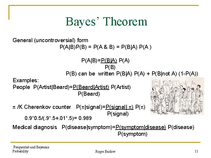
Bayes’ Theorem General (uncontroversial) form P(A|B)P(B) = P(A & B) = P(B|A) P(A|B)=P(B|A) P(B) can be written P(B|A) P(A) + P(B|not A) (1 -P(A)) Examples: People P(Artist|Beard)=P(Beard|Artist) P(Beard) /K Cherenkov counter P( |signal)=P(signal| ) P(signal) 0. 9*0. 5/(. 9*. 5+. 01*. 5)= 0. 989 Medical diagnosis P(disease|symptom)=P(symptom|disease) P(symptom) Frequentist and Bayesian Probability Roger Barlow 11
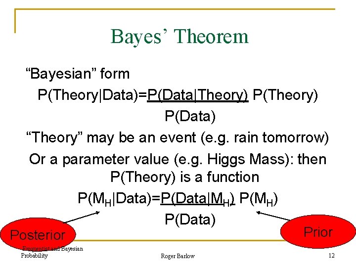
Bayes’ Theorem “Bayesian” form P(Theory|Data)=P(Data|Theory) P(Data) “Theory” may be an event (e. g. rain tomorrow) Or a parameter value (e. g. Higgs Mass): then P(Theory) is a function P(MH|Data)=P(Data|MH) P(Data) Prior Posterior Frequentist and Bayesian Probability Roger Barlow 12
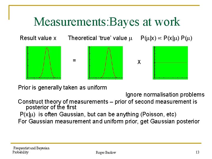
Measurements: Bayes at work Result value x Theoretical ‘true’ value = P( |x) P(x| ) P( ) X Prior is generally taken as uniform Ignore normalisation problems Construct theory of measurements – prior of second measurement is posterior of the first P(x| ) is often Gaussian, but can be anything (Poisson, etc) For Gaussian measurement and uniform prior, get Gaussian posterior Frequentist and Bayesian Probability Roger Barlow 13
Aside: “Objective” Bayesian statistics n Attempt to lay down rule for choice of prior n n n ‘Uniform’ is not enough. Uniform in what? Suggestion (Jeffreys): uniform in a variable for which the expected Fisher information <d 2 ln L/dx 2>is minimum (statisticians call this a ‘flat prior’). Has not met with general agreement – different measurements of the same quantity have different objective priors Frequentist and Bayesian Probability Roger Barlow 14
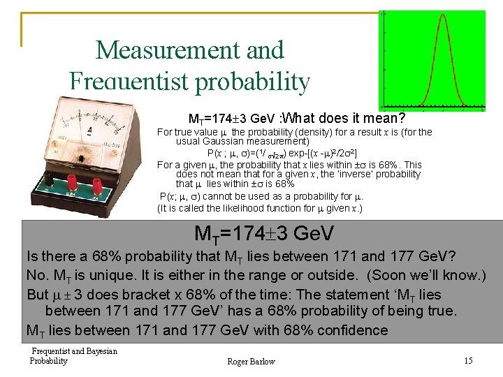
Measurement and Frequentist probability MT=174 3 Ge. V : What does it mean? For true value the probability (density) for a result x is (for the usual Gaussian measurement) P(x ; , )=(1/ 2 ) exp-[(x - )2/2 2] For a given , the probability that x lies within is 68%. This does not mean that for a given x, the ‘inverse’ probability that lies within is 68% P(x; , ) cannot be used as a probability for . (It is called the likelihood function for given x. ) MT=174 3 Ge. V Is there a 68% probability that MT lies between 171 and 177 Ge. V? No. MT is unique. It is either in the range or outside. (Soon we’ll know. ) But 3 does bracket x 68% of the time: The statement ‘MT lies between 171 and 177 Ge. V’ has a 68% probability of being true. MT lies between 171 and 177 Ge. V with 68% confidence Frequentist and Bayesian Probability Roger Barlow 15
Pause for breath For Gaussian measurements of quantities with no constraints/objective prior knowledge the same results are given by: n Frequentist confidence intervals n Bayesian posteriors from uniform priors A frequentist and a simple Bayesian will report the same outcome from the same raw data, except one will say ‘confidence’ and the other ‘probability’. They mean something different but such concerns can be left to the philosophers Frequentist and Bayesian Probability Roger Barlow 16
Frequentist confidence intervals beyond the simple Gaussian Select Confidence Level value CL and strategy From P(x , ) choose construction (functions x 1( ), x 2( )) for which P(x [x 1( ), x 2( )]) CL for all Given a measurement X, make statement [ LO, HI] @ CL Where X=x 2( LO), X=x 1( HI) (Neyman technique) Frequentist and Bayesian Probability Roger Barlow 17
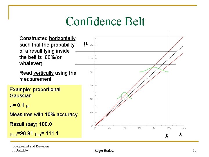
Confidence Belt Constructed horizontally such that the probability of a result lying inside the belt is 68%(or whatever) Read vertically using the measurement Example: proportional Gaussian = 0. 1 Measures with 10% accuracy Result (say) 100. 0 LO=90. 91 HI= 111. 1 Frequentist and Bayesian Probability X Roger Barlow x 18
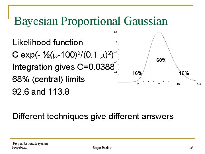
Bayesian Proportional Gaussian Likelihood function C exp(- ½( -100)2/(0. 1 )2) Integration gives C=0. 03888 68% (central) limits 92. 6 and 113. 8 68% 16% Different techniques give different answers Frequentist and Bayesian Probability Roger Barlow 19
Small number counting experiments Poisson distribution P(r; )= e- r / r! For large can use Gaussian approx. But not small Frequentists: Choose CL. Just use one curve to give upper limit Discrete observable makes smooth curves into ugly staircases Observe n. Quote upper limit as HI from solving 0 n P(r, HI) = 0 n e- HI HI r/r! = 1 -CL Translation. n is small. can’t be very large. If the true value is HI (or higher) then the chance of a result this small (or smaller) is only (1 -CL) (or less) Frequentist and Bayesian Probability Roger Barlow 20
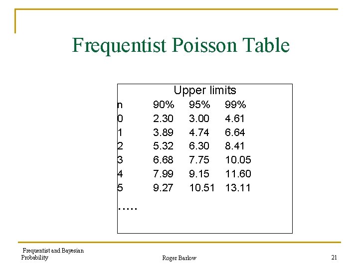
Frequentist Poisson Table Upper limits n 0 1 2 3 4 5 90% 2. 30 3. 89 5. 32 6. 68 7. 99 9. 27 95% 3. 00 4. 74 6. 30 7. 75 9. 15 10. 51 99% 4. 61 6. 64 8. 41 10. 05 11. 60 13. 11 . . . Frequentist and Bayesian Probability Roger Barlow 21
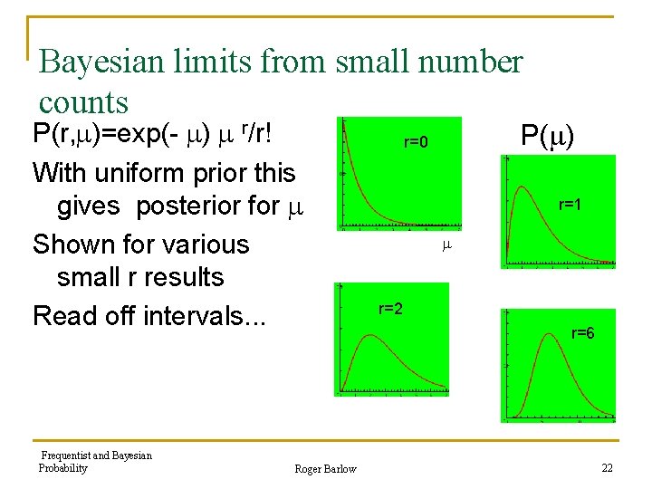
Bayesian limits from small number counts P(r, )=exp(- ) r/r! With uniform prior this gives posterior for Shown for various small r results Read off intervals. . . Frequentist and Bayesian Probability Roger Barlow P( ) r=0 r=1 r=2 r=6 22
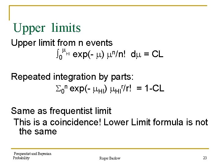
Upper limits Upper limit from n events 0 HI exp(- ) n/n! d = CL Repeated integration by parts: 0 n exp(- HI) HIr/r! = 1 -CL Same as frequentist limit This is a coincidence! Lower Limit formula is not the same Frequentist and Bayesian Probability Roger Barlow 23
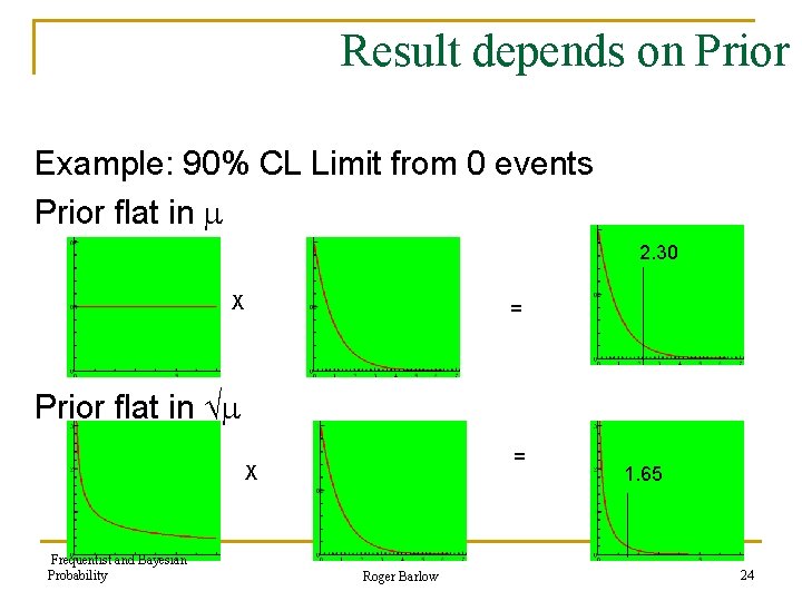
Result depends on Prior Example: 90% CL Limit from 0 events Prior flat in 2. 30 X = Prior flat in = X Frequentist and Bayesian Probability Roger Barlow 1. 65 24
Which is right? n n n Bayesian Method is generally easier, conceptually and in practice Frequentist method is truly objective. Bayesian probability is personal ‘degree of belief’. This does not worry biologists but should worry physicists. Ambiguity appears in Bayesian results as differences in prior give different answers, though with enough data these differences vanish Check for ‘robustnesss under change of prior’ is standard statistical technique, generally ignored by physicists ‘Uniform priors’ is not a sufficient answer. Uniform in what? Frequentist and Bayesian Probability Roger Barlow 25
Problems for Frequentists: Add a background =S+b Frequentist method (b known, measured, S wanted) 1. Find range for 2. Subtract b to get range for S Examples: See 5 events, background 1. 2 95% Upper limit: 10. 5 9. 3 See 5 events, background 5. 1 95% Upper limit: 10. 5 5. 4 ? See 5 events, background 10. 6 95% Upper limit: 10. 5 -0. 1 Frequentist and Bayesian Probability Roger Barlow 26
S< -0. 1? What’s going on? If N<b we know that there is a downward fluctuation in the background. (Which happens…) But there is no way of incorporating this information without messing up the ensemble Really strict frequentist procedure is to go ahead and publish. n We know that 5% of 95%CL statements are wrong – this is one of them n Suppressing this publication will bias the global results Frequentist and Bayesian Probability Roger Barlow 27
Similar problems Expected number of events must be non-negative n Mass of an object must be non-negative n Mass-squared of an object must be non-negative n Higgs mass from EW fits must be bigger than LEP 2 limit of 114 Ge. V 3 Solutions n Publish a ‘clearly crazy’ result n Use Feldman-Cousins technique n Switch to Bayesian analysis n Frequentist and Bayesian Probability Roger Barlow 28
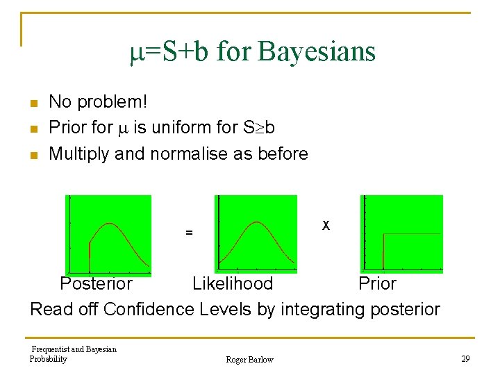
=S+b for Bayesians n n n No problem! Prior for is uniform for S b Multiply and normalise as before X = Posterior Likelihood Prior Read off Confidence Levels by integrating posterior Frequentist and Bayesian Probability Roger Barlow 29
Another Aside: Coverage Given P(x; ) and an ensemble of possible measurements {xi} and some confidence level algorithm, coverage is how often ‘ LO HI’ is true. Isn’t that just the confidence level? Not quite. n Discrete observables may mean the confidence belt is not exact – move on side of caution n Other ‘nuisance’ parameters may need to be taken account of – again erring on side of caution Coverage depends on . For a frequentist it is never less than the CL (‘undercoverage’). It may be more (‘overcoverage’) – this is to be minimised but not crucial For a Bayesian coverage is technically irrelevant – but in practice useful Frequentist and Bayesian Probability Roger Barlow 30
Bayesian pitfall(Heinrich and others) Observe n events from Poisson with = S+b Channel strength S – unknown. Flat prior Efficiency x luminosity - from sub-experiment with flat prior Background b - from sub-experiment with flat prior Investigated coverage and all OK Partition into classes (e. g. different run periods) Coverage falls! Frequentist and Bayesian Probability Roger Barlow 31
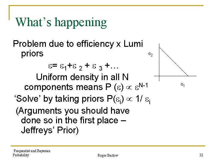
What’s happening Problem due to efficiency x Lumi priors = 1+ 2 + 3 +… Uniform density in all N components means P ( ) N-1 ‘Solve’ by taking priors P( i) 1/ i (Arguments you should have done so in the first place – Jeffreys’ Prior) Frequentist and Bayesian Probability Roger Barlow 2 1 32
Another example: Unitarity triangle Measure CKM angle by measuring B decays (charged and neutral, branching ratios and CP asymmetries). 6 quantities. Many different parametrisations suggested Uniform priors in different parametrisations give different results from each other and from a Frequentist analysis (according to CKMfitter: disputed by UTfit) For a complex number z=x+iy=rei a flat prior in x and y is not the same as a flat prior in r and Frequentist and Bayesian Probability Roger Barlow 33
Loss of ambiguities? Toy example Measure X=( + )2=1. 00 0. 07, Y= 2=1. 10 0. 07 Is interesting but is a nuisance parameter Clearly 4 fold ambiguity 1, 0 or 2 Frequentists stop there Bayesians integrate over and get a peak at 0 double that at 2 – feature persists whatever the prior used for . Is this valid? (Real example will be more subtle) Frequentist and Bayesian Probability Roger Barlow 34
Conclusions Frequentist statistics cannot do everything Bayesian statistics can be dangerous. Choose between 1) Never use it 2) Use only if frequentist method has problems 3) Use only with care and expert guidance and always check for robustness under different priors 4) Use as investigative tool to explore possible interpretations 5) Just plug in the package and write down the results But always know what you are doing and say what you are doing. Frequentist and Bayesian Probability Roger Barlow 35
Backup slides Frequentist and Bayesian Probability Roger Barlow 36
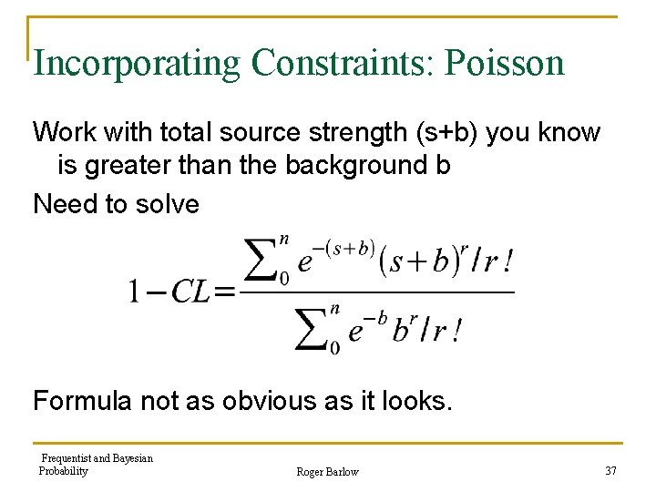
Incorporating Constraints: Poisson Work with total source strength (s+b) you know is greater than the background b Need to solve Formula not as obvious as it looks. Frequentist and Bayesian Probability Roger Barlow 37
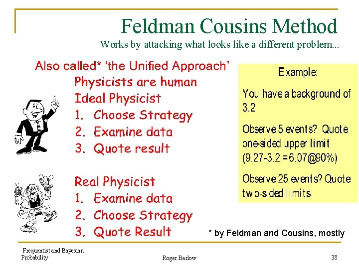
Feldman Cousins Method Works by attacking what looks like a different problem. . . * by Feldman and Cousins, mostly Frequentist and Bayesian Probability Roger Barlow 38
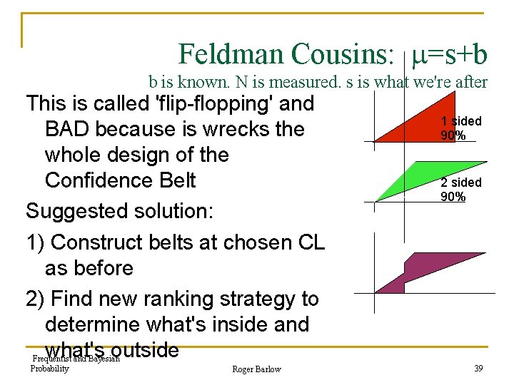
Feldman Cousins: =s+b b is known. N is measured. s is what we're after This is called 'flip-flopping' and BAD because is wrecks the whole design of the Confidence Belt Suggested solution: 1) Construct belts at chosen CL as before 2) Find new ranking strategy to determine what's inside and what's outside Frequentist and Bayesian Probability Roger Barlow 1 sided 90% 2 sided 90% 39
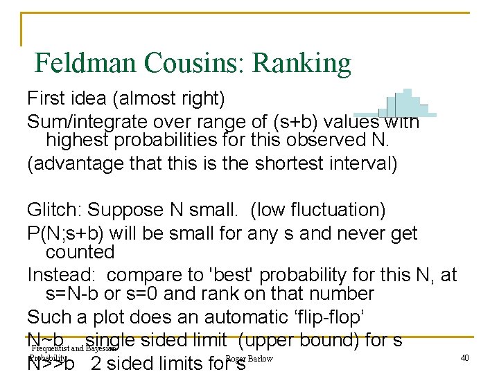
Feldman Cousins: Ranking First idea (almost right) Sum/integrate over range of (s+b) values with highest probabilities for this observed N. (advantage that this is the shortest interval) Glitch: Suppose N small. (low fluctuation) P(N; s+b) will be small for any s and never get counted Instead: compare to 'best' probability for this N, at s=N-b or s=0 and rank on that number Such a plot does an automatic ‘flip-flop’ N~b single sided limit (upper bound) for s Frequentist and Bayesian Probability 40 N>>b 2 sided limits for. Roger s Barlow
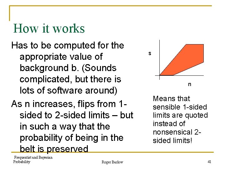
How it works Has to be computed for the appropriate value of background b. (Sounds complicated, but there is lots of software around) As n increases, flips from 1 sided to 2 -sided limits – but in such a way that the probability of being in the belt is preserved Frequentist and Bayesian Probability Roger Barlow s n Means that sensible 1 -sided limits are quoted instead of nonsensical 2 sided limits! 41
Arguments against using Feldman Cousins Argument 1 It takes control out of hands of physicist. You might want to quote a 2 sided limit for an expected process, an upper limit for something weird n Counter argument: This is the virtue of the method. This control invalidates the conventional technique. The physicist can use their discretion over the CL. In rare cases it is permissible to say ”We set a 2 sided limit, but we're not claiming a signal” n Frequentist and Bayesian Probability Roger Barlow 42
Feldman Cousins: Argument 2 If zero events are observed by two experiments, the one with the higher background b will quote the lower limit. This is unfair to hardworking physicists n Counterargument An experiment with higher background has to be ‘lucky’ to get zero events. Luckier experiments will always quote better limits. Averaging over luck, lower values of b get lower limits to report. n Example: you reward a good student with a lottery ticket which has a 10% chance of winning £ 10. A moderate student gets a ticket with a 1% chance of winning £ 20. They both win. Were you unfair? Frequentist and Bayesian Probability Roger Barlow 43
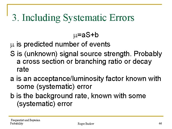
3. Including Systematic Errors =a. S+b is predicted number of events S is (unknown) signal source strength. Probably a cross section or branching ratio or decay rate a is an acceptance/luminosity factor known with some (systematic) error b is the background rate, known with some (systematic) error Frequentist and Bayesian Probability Roger Barlow 44
3. 1 Full Bayesian Assume priors n for S (uniform? ) n For a (Gaussian? ) n For b (Poisson or Gaussian? ) Write down the posterior P(S, a, b). Integrate over all a, b to get marginalised P(s) Read off desired limits by integration Frequentist and Bayesian Probability Roger Barlow 45
3. 2 Hybrid Bayesian Assume priors n For a (Gaussian? ) n For b (Poisson or Gaussian? ) Integrate over all a, b to get marginalised P(r, S) Read off desired limits by 0 n. P(r, S) =1 -CL etc Done approximately for small errors (Cousins and Highland). Shows that limits pretty insensitive to a , b Numerically for general errors (RB: java applet on SLAC web page). Includes 3 priors (for a) that give slightly different results Frequentist and Bayesian Probability Roger Barlow 46
3. 3 -3. 9 Extend Feldman Cousins n Profile Likelihood: Use P(S)=P(n, S, amax, bmax) where amax, bmax give maximum for this S, n n Empirical Bayes n And more… Results being compared as outcome from Banff workshop n Frequentist and Bayesian Probability Roger Barlow 47
Summary n n n Straight Frequentist approach is objective and clean but sometimes gives ‘crazy’ results Bayesian approach is valuable but has problems. Check for robustness under choice of prior Feldman-Cousins deserves more widespread adoption Lots of work still going on This will all be needed at the LHC Frequentist and Bayesian Probability Roger Barlow 48
- Slides: 48