Probability Distributions Random variables can be discrete or

Probability Distributions

Random variables can be discrete or continuous n Discrete random variables have a countable number of outcomes n n Examples: Dead/alive, treatment/placebo, dice, counts, etc. Continuous random variables have an infinite continuum of possible values. n Examples: blood pressure, weight, the speed of a car, the real numbers from 1 to 6.

Probability functions n n n A probability function maps the possible values of x against their respective probabilities of occurrence, p(x) is a number from 0 to 1. 0. The area under a probability function is always 1.

Discrete example 1 Toss a fair coin three times and define x = number of heads.

Discrete example 2 Toss two dice and define x = sum of two dice. x p(x) 2 1/36 3 2/36 4 3/36 5 4/36 6 5/36 7 6/36 8 5/36 9 4/36 10 3/36 11 2/36 12 1/36

Discrete example 3: roll of a die x p(x) 1 p(x=1)=1/6 2 p(x=2)=1/6 3 p(x=3)=1/6 4 p(x=4)=1/6 5 p(x=5)=1/6 6 p(x=6)=1/6 1. 0

Discrete example 3: roll of a die p(x) 1/6 1 2 3 4 5 6 x

Discrete example 4: roll of a die x P(x≤A) 1 P(x≤ 1)=1/6 2 P(x≤ 2)=2/6 3 P(x≤ 3)=3/6 4 P(x≤ 4)=4/6 5 P(x≤ 5)=5/6 6 P(x≤ 6)=6/6

Discrete example 4: roll of a die 1. 0 5/6 2/3 1/2 1/3 1/6 P(x) 1 2 3 4 5 6 x

Examples 1. What’s the probability that you roll a 3 or less? P(x≤ 3)=1/2 2. What’s the probability that you roll a 5 or higher? P(x≥ 5) = 1 – P(x≤ 4) = 1 -2/3 = 1/3

Practice Problem: n The number of ships to arrive at a harbor on any given day is a random variable represented by x. The probability distribution for x is: x P(x) 10. 4 11. 2 12. 2 13. 1 14. 1 Find the probability that on a given day: a. exactly 14 ships arrive b. At least 12 ships arrive p(x 12)= (. 2 +. 1) =. 4 c. At most 11 ships arrive p(x≤ 11)= (. 4 +. 2) =. 6 p(x=14)=. 1

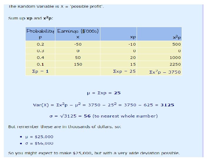
The Mean and Standard Deviation n Let x be a discrete random variable with probability distribution p(x). Then the mean, variance and standard deviation of x are given as

Standard Deviation n The Standard Deviation is a measure of how spread out numbers are. Its symbol is σ (the greek letter sigma) The formula is easy: it is the square root of the Variance. So now you ask, "What is the Variance? "

Variance n The Variance is defined as: To calculate the variance follow these steps: n n n Work out the Mean (the simple average of the numbers) Then for each number: subtract the Mean and square the result (the squared difference). Then work out the average of those squared differences.

Example n You have just measured the heights of below dogs (in millimeters):

Answer:

For example, bell-curve (normal) distribution: Mean ( ) One standard deviation from the mean ( )

Example § Toss a fair coin 3 times and record x the number of heads.

Example § The probability distribution for x the number of heads in tossing 3 fair coins.

Example: expected value n Recall the following probability distribution of ship arrivals: x P(x) 10. 4 11. 2 12. 2 13. 1 14. 1

Expected value, formally Discrete case: Continuous case:

Extension to continuous case: uniform distribution p(x) 1 1 x

Variance, formally Discrete case: Continuous case:

Handy calculation formula! Handy calculation formula (if you ever need to calculate by hand!): Intervening algebra!

Var(x) = E(x- )2 = E(x 2) – [E(x)]2 (your calculation formula!) Proofs (optional!): E(x- )2 = E(x 2– 2 x + 2) =E(x 2) – E(2 x) +E( 2) = E(x 2) – 2 E(x) + 2 = E(x 2) – [E(x)]2 OR, equivalently: E(x- )2 = remember “FOIL”? ! Use rules of expected value: E(X+Y)= E(X) + E(Y) E(c) = c E(x) =

For example, what’s the variance and standard deviation of the roll of a die? 1 x p(x) p(x=1)=1/6 2 p(x=2)=1/6 3 p(x=3)=1/6 4 p(x=4)=1/6 5 p(x=5)=1/6 6 p(x=6)=1/6 1. 0 p(x) average distance from the mean 1/6 1 2 3 4 5 6 mean x

Var(c) = 0 Constants don’t vary!

Practice Problem Find the variance and standard deviation for the number of ships to arrive at the harbor (recall that the mean is 11. 3). x P(x) 10. 4 11. 2 12. 2 13. 1 14. 1

Answer: variance and std dev x 2 P(x) 100. 4 121. 2 144. 2 169. 1 196. 1 Interpretation: On an average day, we expect 11. 3 ships to arrive in the harbor, plus or minus 1. 35. This gives you a feel for what would be considered a usual day!

Practice Problem You toss a coin 100 times. What’s the expected number of heads? What’s the variance of the number of heads?

Answer: expected value Intuitively, we’d probably all agree that we expect around 50 heads, right? Another way to show this Think of tossing 1 coin. E(X=number of heads) = (1) P(heads) + (0)P(tails) E(X=number of heads) = 1(. 5) + 0 =. 5 If we do this 100 times, we’re looking for the sum of 100 tosses, where we assign 1 for a heads and 0 for a tails. (these are 100 “independent, identically distributed (i. i. d)” events) E(X 1 +X 2 +X 3 +X 4 +X 5 …. . +X 100) = E(X 1) + E(X 2) + E(X 3)+ E(X 4)+ E(X 5) …. . + E(X 100) = 100 E(X 1) = 50

Answer: variance What’s the variability, though? More tricky. But, again, we could do this for 1 coin and then use our rules of variance. Think of tossing 1 coin. E(X 2=number of heads squared) = 12 P(heads) + 02 P(tails) E(X 2) = 1(. 5) + 0 =. 5 Var(X) =. 5 -. 52 =. 5 -. 25 =. 25 Then, using our rule: Var(X+Y)= Var(X) + Var(Y) (coin tosses are independent!) Var(X 1 +X 2 +X 3 +X 4 +X 5 …. . +X 100) = Var(X 1) + Var(X 2) + Var(X 3)+ Var(X 4)+ Var(X 5) …. . + Var(X 100) = 100 Var(X 1) = 100 (. 25) = 25 SD(X)=5 Interpretation: When we toss a coin 100 times, we expect to get 50 heads plus or minus 5.

Example

Continuous Probability Distribution n Suppose we measure height of students in this class. If we “discretize” by rounding to the nearest feet, the discrete probability histogram is shown on the left. Now if height is measured to the nearest inch, a possible probability histogram is shown in the middle. We get more bins and much smoother appearance. Imagine we continue in this way to measure height more and more finely, the resulting probability histograms approach a smooth curve shown on the right.

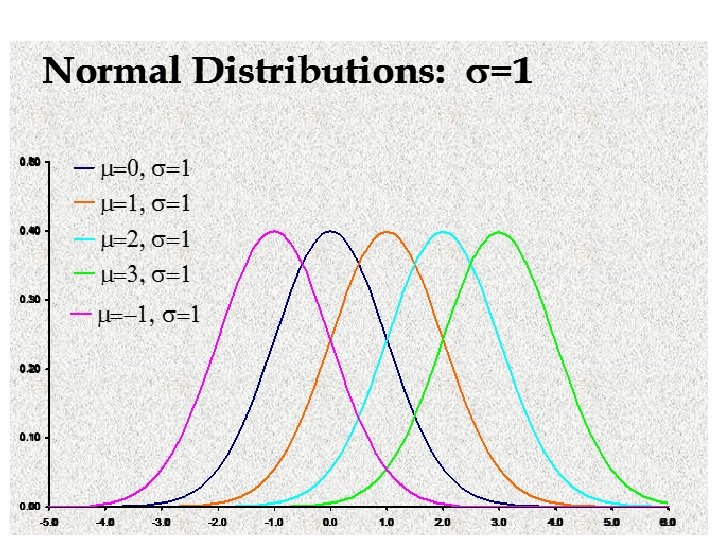
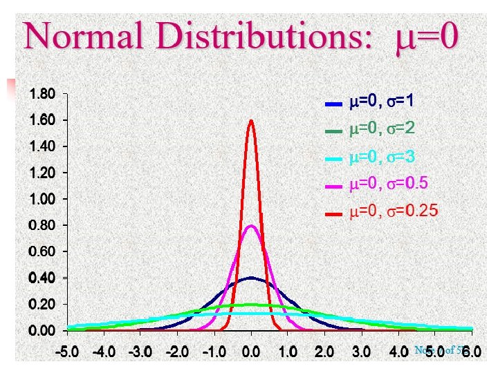
The Normal Distribution n The formula that generates the normal probability distribution is: Two parameters, mean and standard deviation, completely determine the Normal distribution. The shape and location of the normal curve changes as the mean and standard deviation change.

The Normal Distribution Many things closely follow a Normal Distribution: n heights of people n size of things produced by machines n errors in measurements n blood pressure n marks on a test

The Standard Normal Distribution n n To find P(a < x < b), we need to find the area under the appropriate normal curve. To simplify the tabulation of these areas, we standardize each value of x by expressing it as a z-score, the number of standard deviations s it lies from the mean .