Probability Distributions Objectives Understand the attributes and applications

Probability Distributions

Objectives • Understand the attributes and applications of the binomial distribution • Understand the attributes and applications of the normal distribution • Understand apply the results of the Central Limit Theorem

Probability Requirements • Requirements for the probability distribution of a discrete random variable x: 1. P(x) 0 for all values of x 2. p(x) = 1 All x
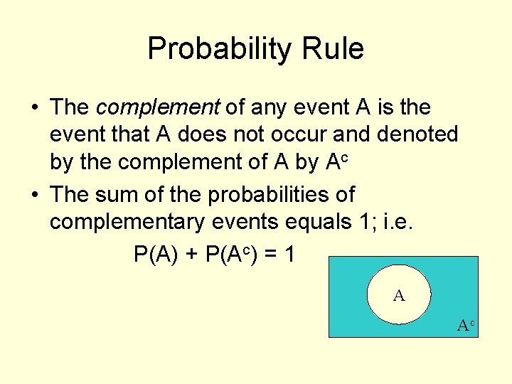
Probability Rule • The complement of any event A is the event that A does not occur and denoted by the complement of A by Ac • The sum of the probabilities of complementary events equals 1; i. e. P(A) + P(Ac) = 1 A Ac

Random Variable • A rule that assigns one and only one numerical value to each simple event of an experiment. • Random variable that can assume a countable number of values are called Discrete.
Random Variable • Random variable that can assume value corresponding to any of the points contained in one or more intervals are called continuous
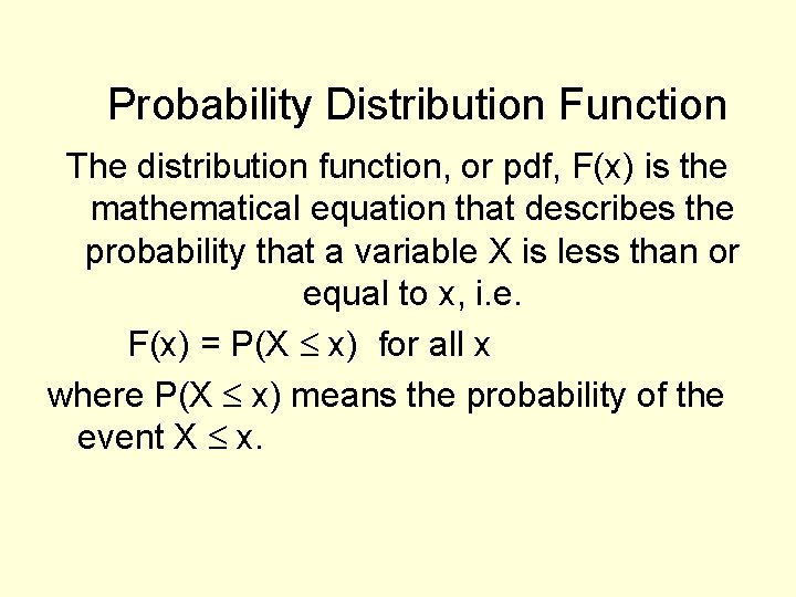
Probability Distribution Function The distribution function, or pdf, F(x) is the mathematical equation that describes the probability that a variable X is less than or equal to x, i. e. F(x) = P(X x) for all x where P(X x) means the probability of the event X x.
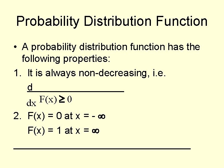
Probability Distribution Function • A probability distribution function has the following properties: 1. It is always non-decreasing, i. e. d dx F(x) 0 2. F(x) = 0 at x = - F(x) = 1 at x =
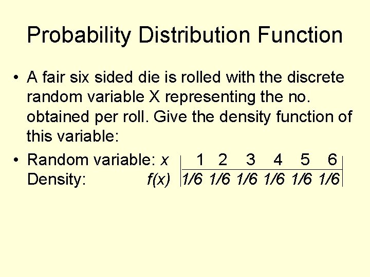
Probability Distribution Function • A fair six sided die is rolled with the discrete random variable X representing the no. obtained per roll. Give the density function of this variable: • Random variable: x 1 2 3 4 5 6 Density: f(x) 1/6 1/6 1/6
Probability Distribution • The probability of a discrete random variable is a graph, table, or formula that specifies the probability associated with each possible value the random variable can assume.
Binomial Distribution • Binomial distribution is encountered in nature when an event can occur in one of only two mutually exclusive way. • For example: the distribution of the number of female rats in litter of size is binomial because each rat must be either male or female (excluding the rare hermaphrodite).
Binomial Distribution • Model for discrete outcome • Process or experiment has 2 possible outcomes: success and failure • Replications of process are independent • P(success) is constant for each replication
Binomial Distribution • Coin tossing is another example of binomial distribution, everytime a coin is tossed the outcome can only be either head or tail.
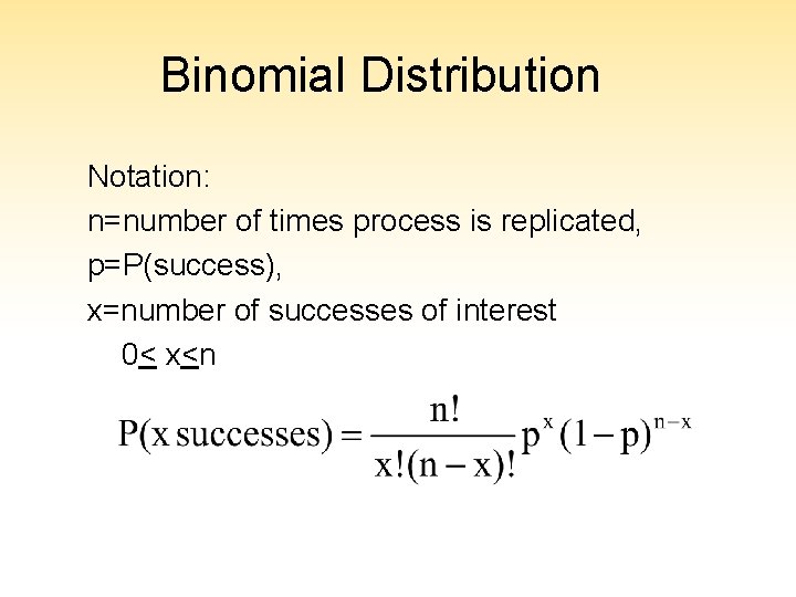
Binomial Distribution Notation: n=number of times process is replicated, p=P(success), x=number of successes of interest 0< x<n
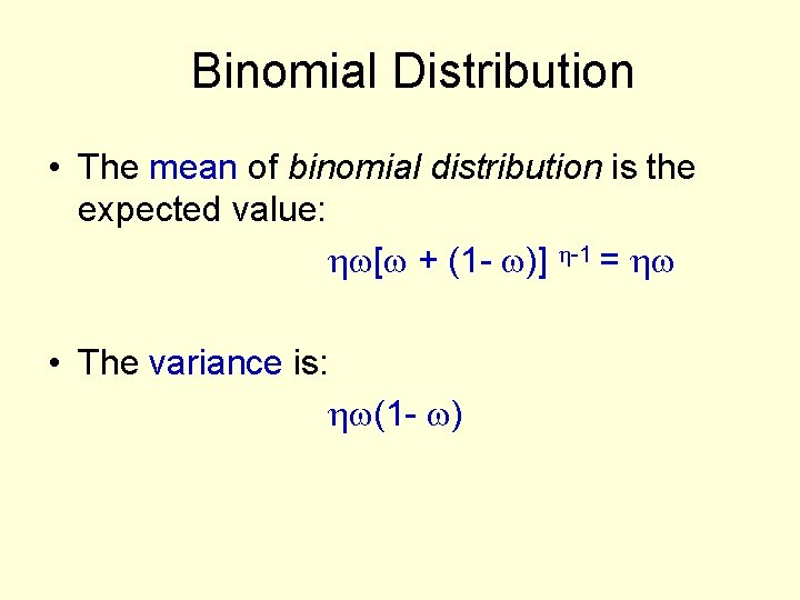
Binomial Distribution • The mean of binomial distribution is the expected value: [ + (1 - )] -1 = • The variance is: (1 - )
![Binomial Distribution [ =12, = 0. 5] Binomial Distribution [ =12, = 0. 5]](http://slidetodoc.com/presentation_image_h/0f7c46c553c91e03ee6cc2024ef324fe/image-16.jpg)
Binomial Distribution [ =12, = 0. 5]
Binomial Distribution • The fundamental assumption of a binomial distribution is that the probability of success of a trial is independent of the outcome of any previous trials, i. e. , each trial is independent. • The success of a trial can not improve or deteriorate depending on the results of previous trials.
Binomial Distribution • In some cases binomial distribution can be approximated by using other distributions for which computations are less laborious. • For example for small and large , the Poisson distribution may be appropriate.
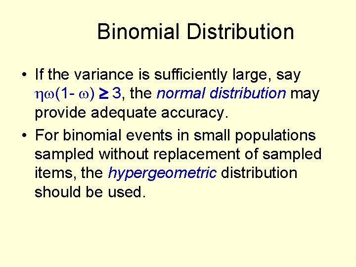
Binomial Distribution • If the variance is sufficiently large, say (1 - ) 3, the normal distribution may provide adequate accuracy. • For binomial events in small populations sampled without replacement of sampled items, the hypergeometric distribution should be used.
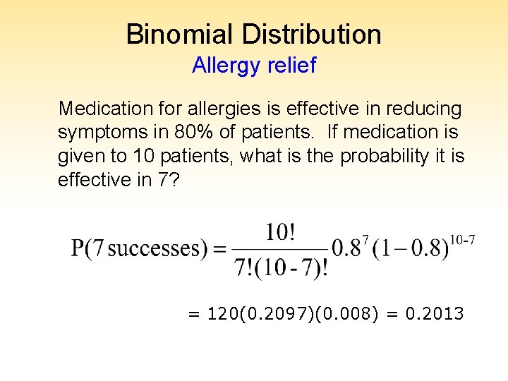
Binomial Distribution Allergy relief Medication for allergies is effective in reducing symptoms in 80% of patients. If medication is given to 10 patients, what is the probability it is effective in 7? = 120(0. 2097)(0. 008) = 0. 2013
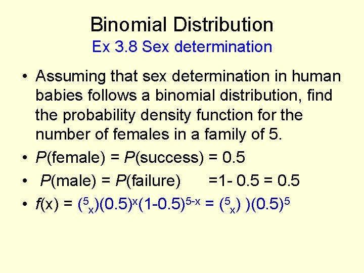
Binomial Distribution Ex 3. 8 Sex determination • Assuming that sex determination in human babies follows a binomial distribution, find the probability density function for the number of females in a family of 5. • P(female) = P(success) = 0. 5 • P(male) = P(failure) =1 - 0. 5 = 0. 5 • f(x) = (5 x)(0. 5)x(1 -0. 5)5 -x = (5 x) )(0. 5)5
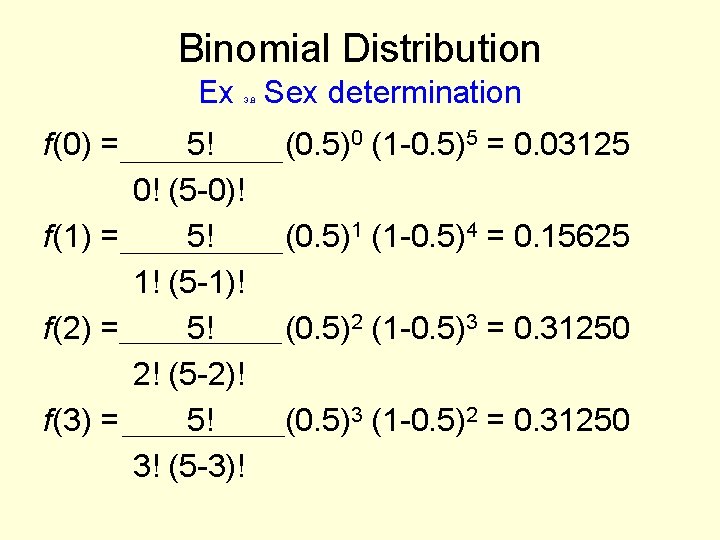
Binomial Distribution Ex Sex determination 3. 8 f(0) = 5! 0! (5 -0)! f(1) = 5! 1! (5 -1)! f(2) = 5! 2! (5 -2)! f(3) = 5! 3! (5 -3)! (0. 5)0 (1 -0. 5)5 = 0. 03125 (0. 5)1 (1 -0. 5)4 = 0. 15625 (0. 5)2 (1 -0. 5)3 = 0. 31250 (0. 5)3 (1 -0. 5)2 = 0. 31250
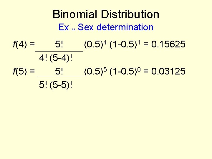
Binomial Distribution Ex Sex determination 3. 8 f(4) = 5! 4! (5 -4)! f(5) = 5! 5! (5 -5)! (0. 5)4 (1 -0. 5)1 = 0. 15625 (0. 5)5 (1 -0. 5)0 = 0. 03125
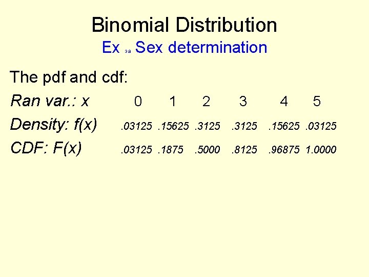
Binomial Distribution Ex Sex determination 3. 8 The pdf and cdf: Ran var. : x 0 Density: f(x). 03125 CDF: F(x). 03125 1 2 3 4 5 . 15625. 3125 . 15625. 03125 . 1875 . 8125 . 96875 1. 0000 . 5000
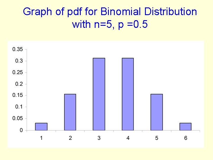
Graph of pdf for Binomial Distribution with n=5, p =0. 5
Normal Distribution
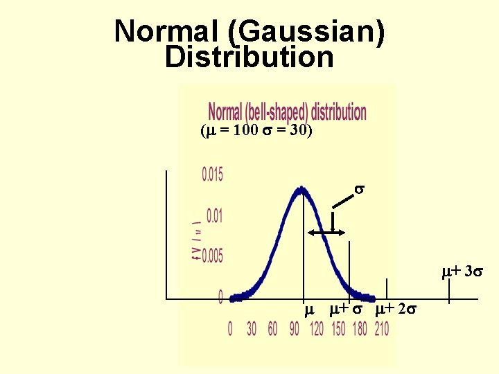
Normal (Gaussian) Distribution • This continuous distribution formulated by Gauss et. al. has come to be known as normal distribution because it can be used to approximate closely the behavior of large number of natural random variable that are continuous. • For example the weight of Holstein Friesian cows, the height of American young males, etc.
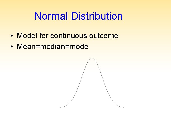
Normal Distribution • Model for continuous outcome • Mean=median=mode
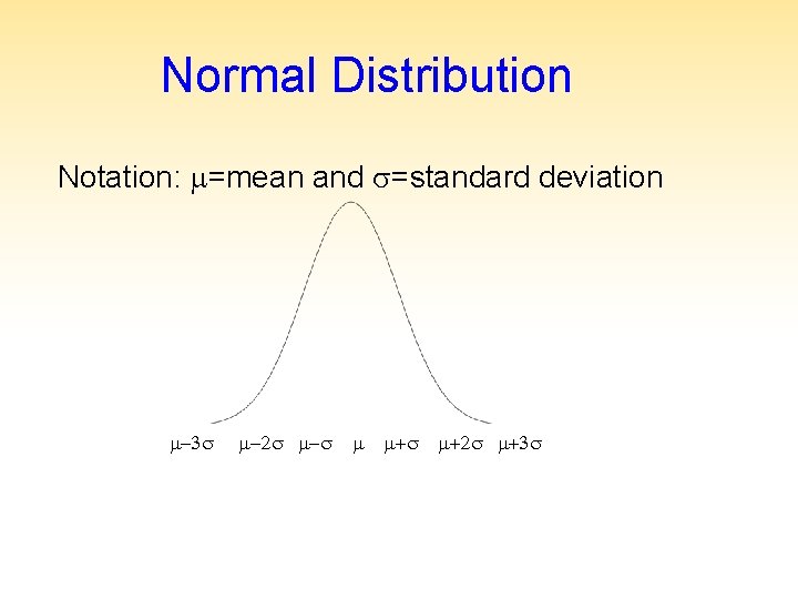
Normal Distribution Notation: =mean and =standard deviation -3 -2 - + +2 +3
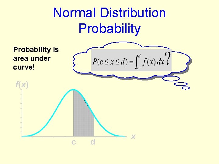
Normal Distribution Probability is area under curve!
Normal (Gaussian) Distribution • The strongest justification for normal distribution come from the central limit theorem which state: If a population has finite variance 2 and mean for the random variable Y, the distribution of the sample mean approaches the normal distribution with variance 2/n and mean as the sample size n increases, regardless of the form of the distribution of Y.
Normal (Gaussian) Distribution • For a continuous random variable Y, the normal density function is: f. Y(y) = (1/ 2 2)e-(y- )2/2 2 (- < y < + ) • Note that the distribution of any specific variable depends on only two parameters, mean and variance 2
Normal (Gaussian) Distribution • The distributions of some of the continuous biological variates may not closely correspond to the normal distribution. • Two common measures of deviation from normality are skewness and kurtosis.
Normal (Gaussian) Distribution ( = 100 = 30) + 3 + + 2
Normal (Gaussian) Distribution Normal (0, 1) Normal (0, 1. 6) -5 -2. 5 0 2. 5 5
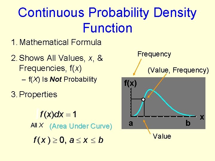
Continuous Probability Density Function 1. Mathematical Formula Frequency 2. Shows All Values, x, & Frequencies, f(x) – f(X) Is Not Probability (Value, Frequency) f(x) 3. Properties f ( x )dx 1 All X (Area Under Curve) f ( x ) 0, a x b a b Value x
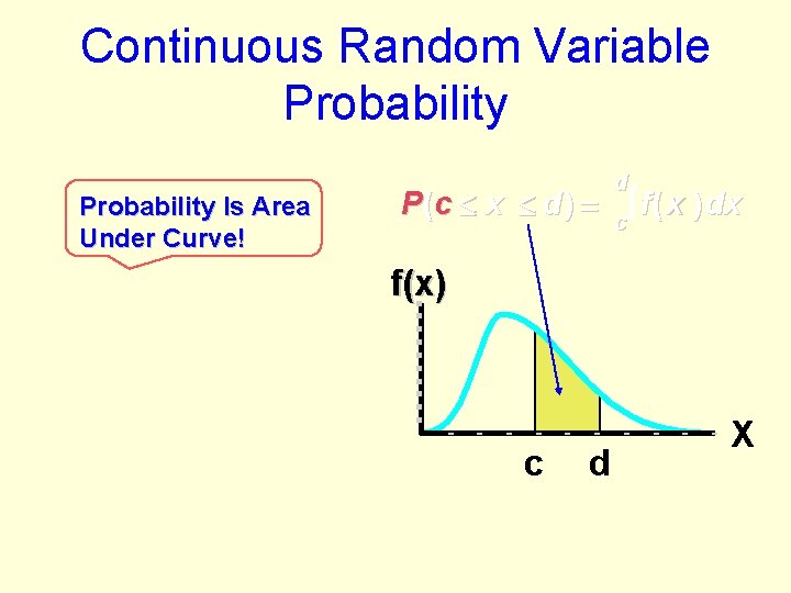
Continuous Random Variable Probability Is Area Under Curve! d P (c x d) c f ( x ) dx f(x) c © 1984 -1994 T/Maker Co. d X
Importance of Normal Distribution 1. Describes Many Random Processes or Continuous Phenomena 2. Can Be Used to Approximate Discrete Probability Distributions – Example: Binomial 3. Basis for Classical Statistical Inference
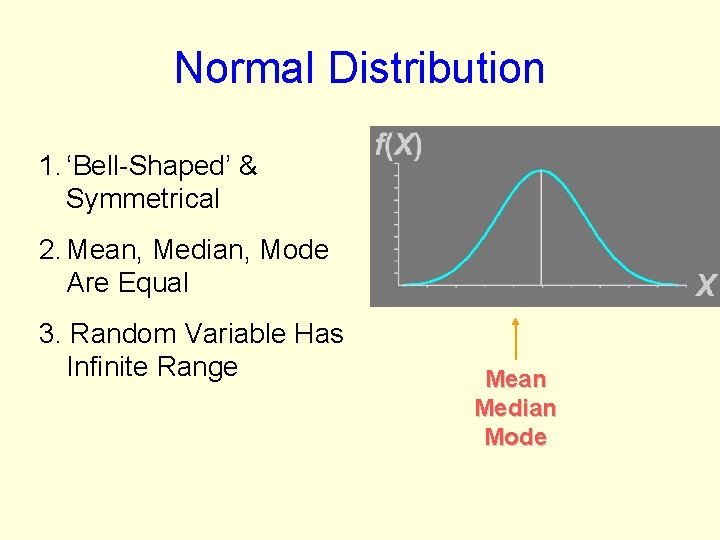
Normal Distribution 1. ‘Bell-Shaped’ & Symmetrical 2. Mean, Median, Mode Are Equal 3. Random Variable Has Infinite Range Mean Median Mode
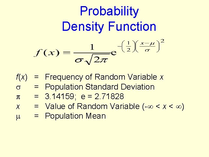
Probability Density Function f(x) x = = = Frequency of Random Variable x Population Standard Deviation 3. 14159; e = 2. 71828 Value of Random Variable (- < x < ) Population Mean
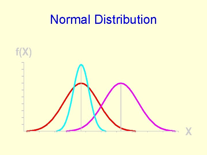
Normal Distribution
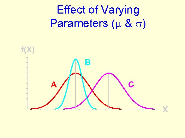
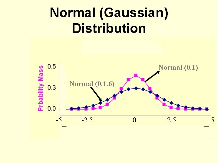
Effect of Varying Parameters ( & )
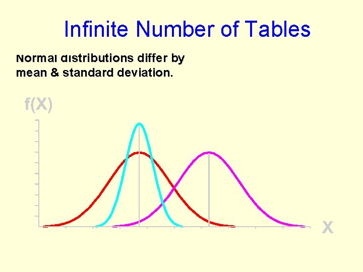
Infinite Number of Tables Normal distributions differ by mean & standard deviation.
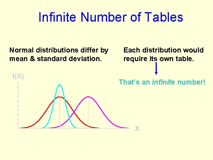
Infinite Number of Tables Normal distributions differ by mean & standard deviation. Each distribution would require its own table. That’s an infinite number!
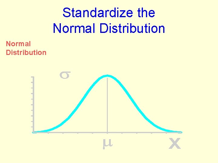
Standardize the Normal Distribution
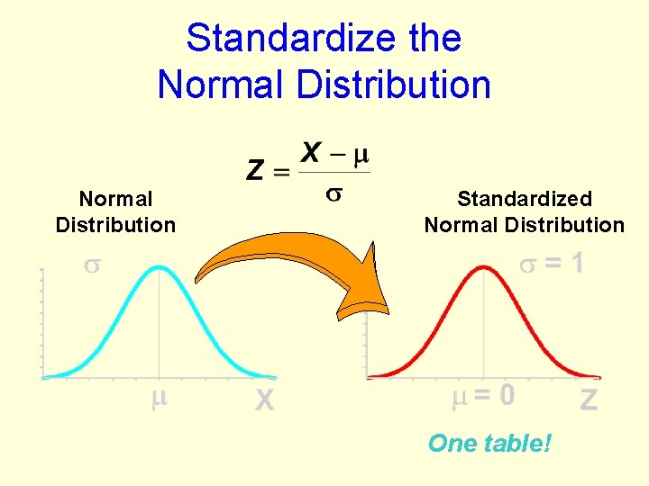
Standardize the Normal Distribution Standardized Normal Distribution One table!
Intuitions on Standardizing • Subtracting Mu from each value X just moves the curve around, so values are centered on 0 instead of on Mu • Once the curve is centered, dividing each value by sigma>1 moves all values toward 0, smushing the curve
Normal Distribution Body mass index (BMI) for men age 60 is normally distributed with a mean of 29 and standard deviation of 6? What is the probability that a male has BMI less than 35?
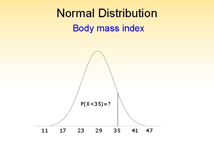
Normal Distribution Body mass index P(X<35)=? 11 17 23 29 35 41 47
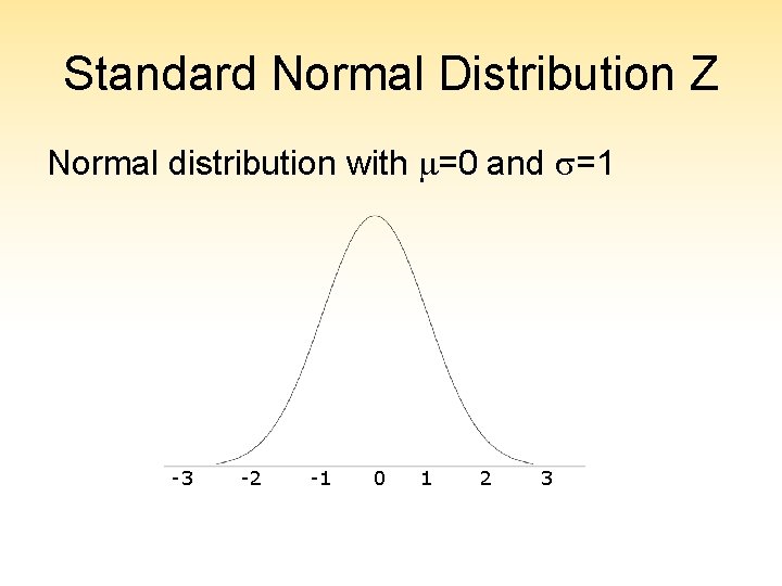
Standard Normal Distribution Z Normal distribution with =0 and =1 -3 -2 -1 0 1 2 3
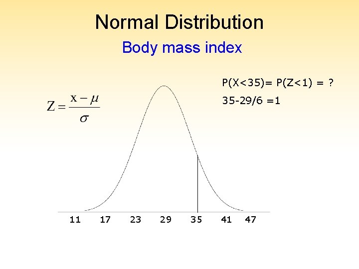
Normal Distribution Body mass index P(X<35)= P(Z<1) = ? 35 -29/6 =1 11 17 23 29 35 41 47
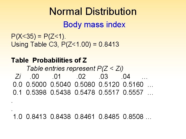
Normal Distribution Body mass index P(X<35) = P(Z<1). Using Table C 3, P(Z<1. 00) = 0. 8413 Table Probabilities of Z Table entries represent P(Z < Zi) Zi. 00. 01. 02. 03. 04 … 0. 0 0. 5000 0. 5040 0. 5080 0. 5120 0. 5160 … 0. 1 0. 5398 0. 5438 0. 5478 0. 5517 0. 5557 …. . 1. 0 0. 8413 0. 8438 0. 8461 0. 8485 0. 8508 …
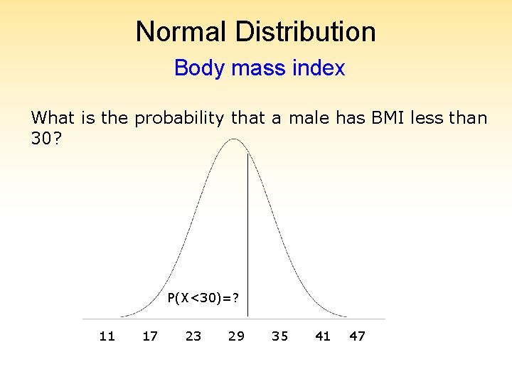
Normal Distribution Body mass index What is the probability that a male has BMI less than 30? P(X<30)=? 11 17 23 29 35 41 47
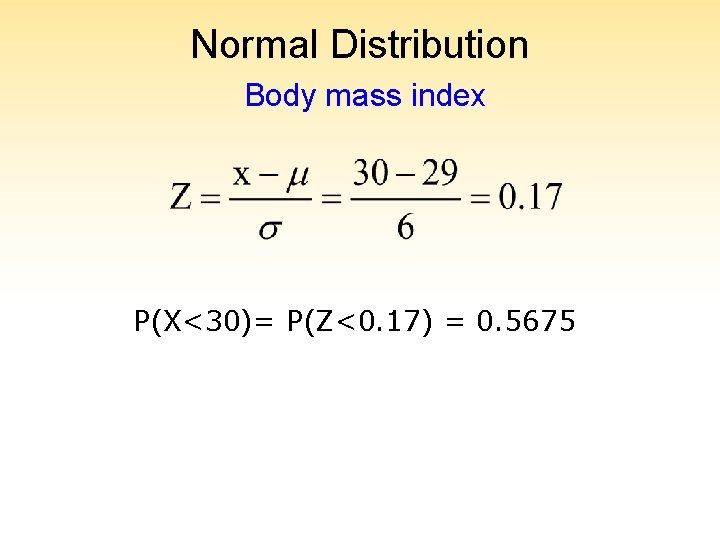
Normal Distribution Body mass index P(X<30)= P(Z<0. 17) = 0. 5675
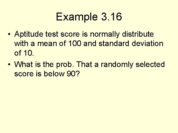
Example 3. 16 • Aptitude test score is normally distribute with a mean of 100 and standard deviation of 10. • What is the prob. That a randomly selected score is below 90?
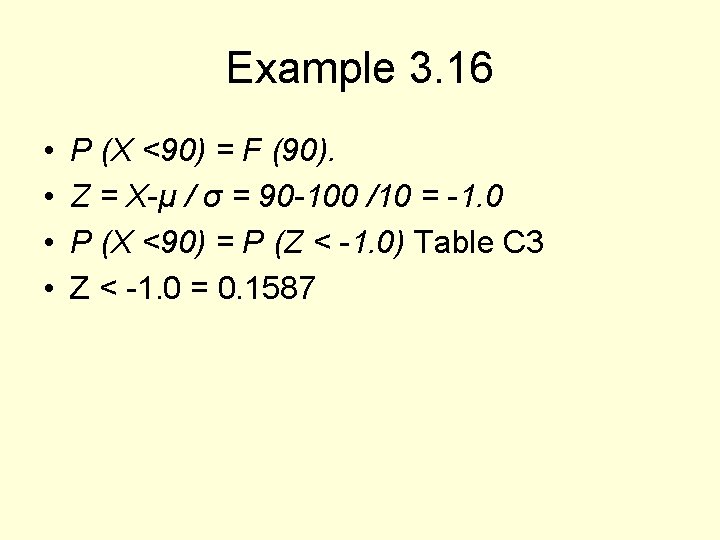
Example 3. 16 • • P (X <90) = F (90). Z = X-μ / σ = 90 -100 /10 = -1. 0 P (X <90) = P (Z < -1. 0) Table C 3 Z < -1. 0 = 0. 1587
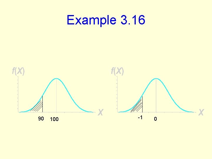
Example 3. 16 90 100 -1 0
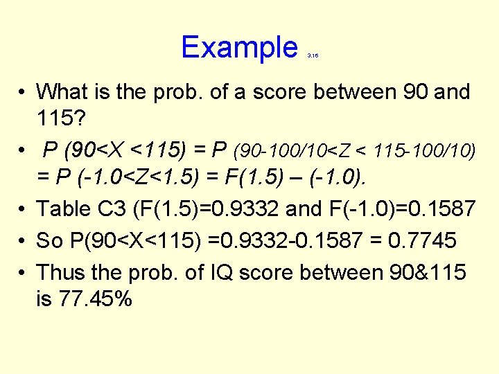
Example 3. 16 • What is the prob. of a score between 90 and 115? • P (90<X <115) = P (90 -100/10<Z < 115 -100/10) = P (-1. 0<Z<1. 5) = F(1. 5) – (-1. 0). • Table C 3 (F(1. 5)=0. 9332 and F(-1. 0)=0. 1587 • So P(90<X<115) =0. 9332 -0. 1587 = 0. 7745 • Thus the prob. of IQ score between 90&115 is 77. 45%
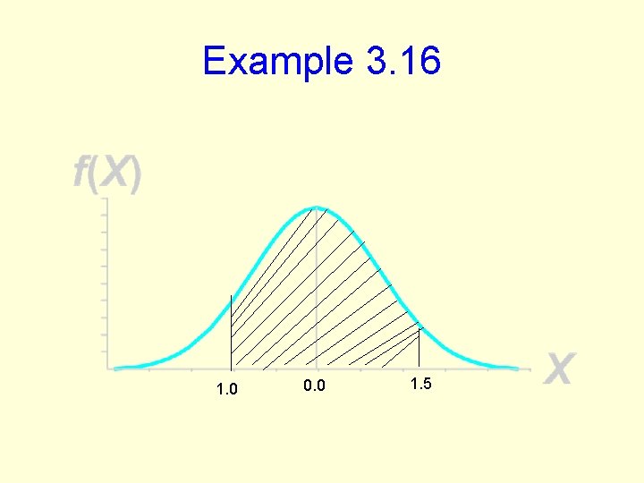
Example 3. 16 1. 0 0. 0 1. 5
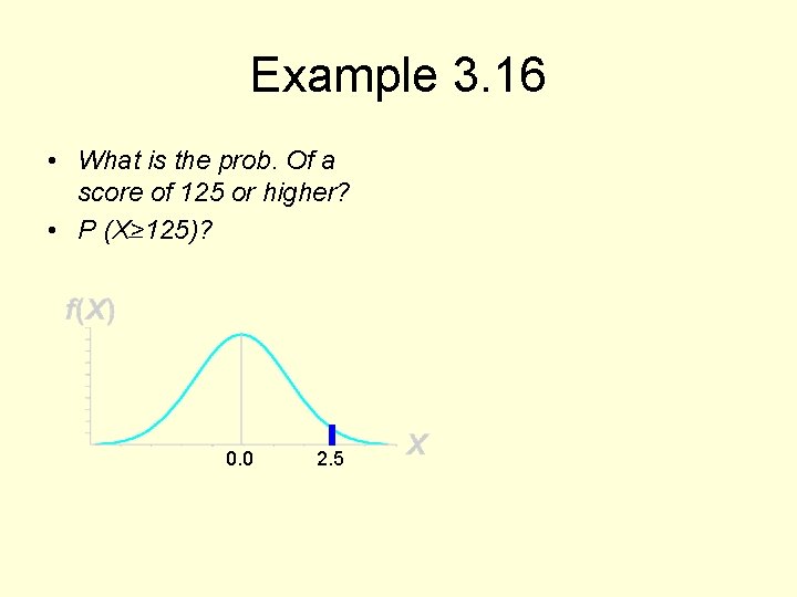
Example 3. 16 • What is the prob. Of a score of 125 or higher? • P (X>125)? 0. 0 2. 5
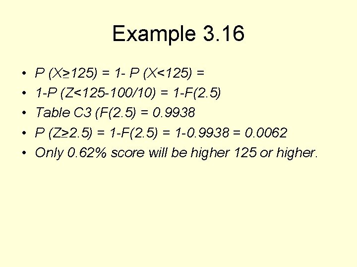
Example 3. 16 • • • P (X>125) = 1 - P (X<125) = 1 -P (Z<125 -100/10) = 1 -F(2. 5) Table C 3 (F(2. 5) = 0. 9938 P (Z>2. 5) = 1 -F(2. 5) = 1 -0. 9938 = 0. 0062 Only 0. 62% score will be higher 125 or higher.
Percentiles of the Normal Distribution • A percentile is a value that holds a specified percentage of the distribution below it. • The median is the 50 th percentile, Q 1 is the 25 th percentile and Q 3 is the 75 th percentile.
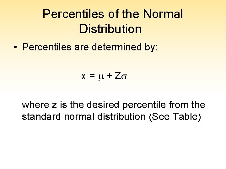
Percentiles of the Normal Distribution • Percentiles are determined by: x = + Z where z is the desired percentile from the standard normal distribution (See Table)
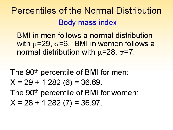
Percentiles of the Normal Distribution Body mass index BMI in men follows a normal distribution with =29, =6. BMI in women follows a normal distribution with =28, =7. The 90 th percentile of BMI for men: X = 29 + 1. 282 (6) = 36. 69. The 90 th percentile of BMI for women: X = 28 + 1. 282 (7) = 36. 97.
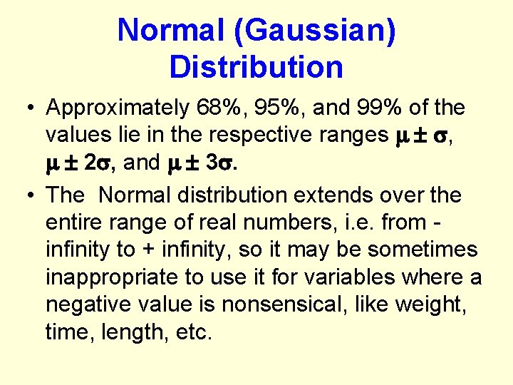
Normal (Gaussian) Distribution • Approximately 68%, 95%, and 99% of the values lie in the respective ranges , 2 , and 3. • The Normal distribution extends over the entire range of real numbers, i. e. from infinity to + infinity, so it may be sometimes inappropriate to use it for variables where a negative value is nonsensical, like weight, time, length, etc.
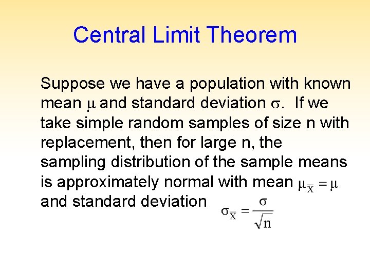
Central Limit Theorem Suppose we have a population with known mean and standard deviation . If we take simple random samples of size n with replacement, then for large n, the sampling distribution of the sample means is approximately normal with mean and standard deviation
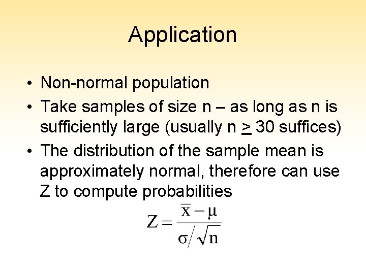
Application • Non-normal population • Take samples of size n – as long as n is sufficiently large (usually n > 30 suffices) • The distribution of the sample mean is approximately normal, therefore can use Z to compute probabilities
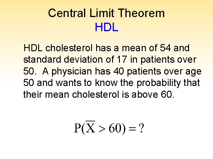
Central Limit Theorem HDL cholesterol has a mean of 54 and standard deviation of 17 in patients over 50. A physician has 40 patients over age 50 and wants to know the probability that their mean cholesterol is above 60.
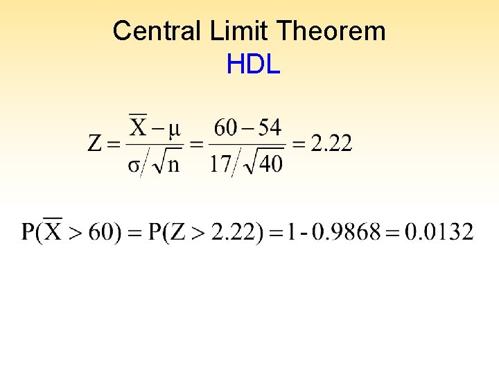
Central Limit Theorem HDL
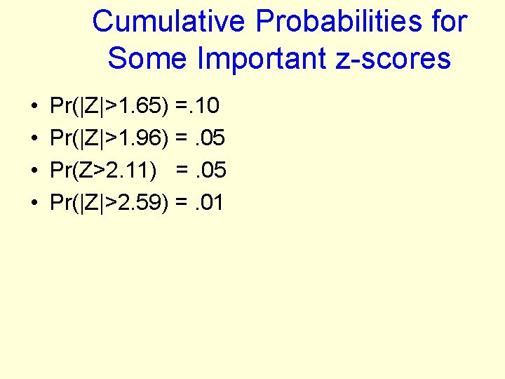
Cumulative Probabilities for Some Important z-scores • • Pr(|Z|>1. 65) =. 10 Pr(|Z|>1. 96) =. 05 Pr(Z>2. 11) =. 05 Pr(|Z|>2. 59) =. 01
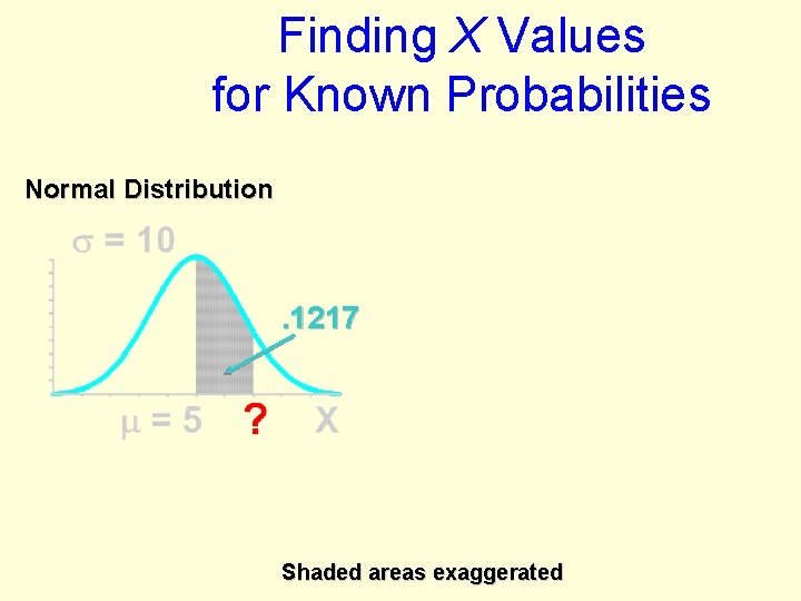
Finding X Values for Known Probabilities Normal Distribution . 1217 Shaded areas exaggerated
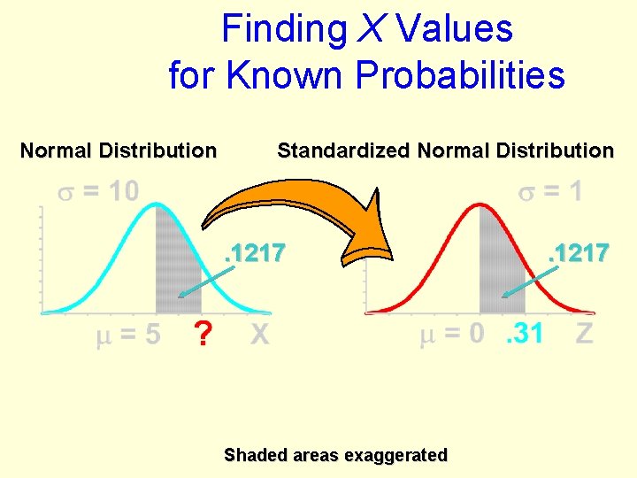
Finding X Values for Known Probabilities Normal Distribution Standardized Normal Distribution . 1217 Shaded areas exaggerated . 1217
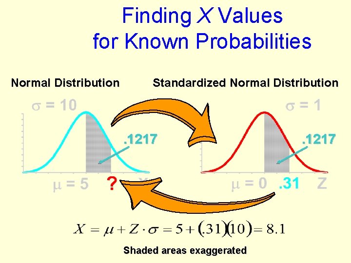
Finding X Values for Known Probabilities Normal Distribution Standardized Normal Distribution . 1217 Shaded areas exaggerated . 1217
Normal Approximation of Binomial Distribution
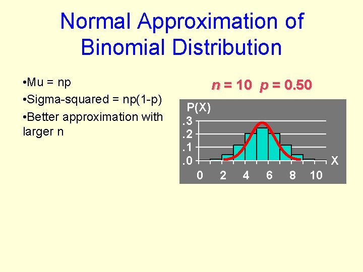
Normal Approximation of Binomial Distribution • Mu = np • Sigma-squared = np(1 -p) • Better approximation with larger n n = 10 p = 0. 50 P(X). 3. 2. 1. 0 0 2 X 4 6 8 10
- Slides: 75