Probability Distributions Chapter 7 Random Variables A Random

Probability Distributions Chapter 7

Random Variables A Random variable assigns a number to each outcome of a random circumstance, or equivalently, a random variable assigns a number to each unit in a population.

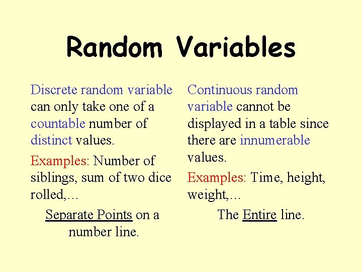
Random Variables Discrete random variable can only take one of a countable number of distinct values. Examples: Number of siblings, sum of two dice rolled, … Separate Points on a number line. Continuous random variable cannot be displayed in a table since there are innumerable values. Examples: Time, height, weight, … The Entire line.

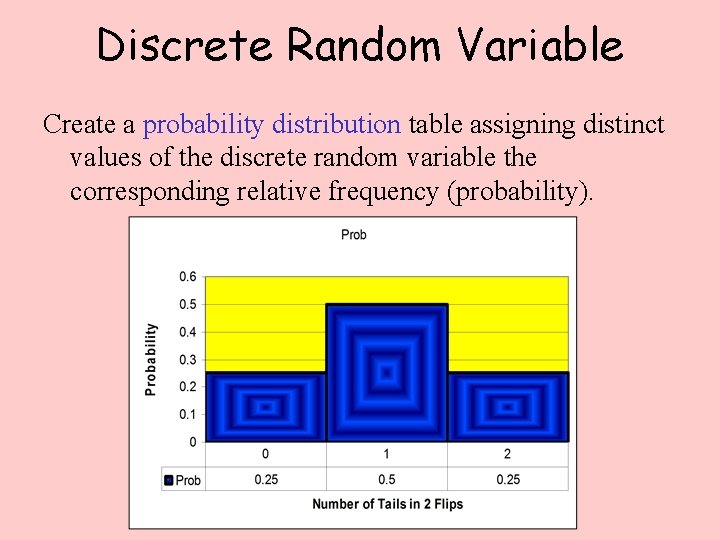
Discrete Random Variable Create a probability distribution table assigning distinct values of the discrete random variable the corresponding relative frequency (probability).

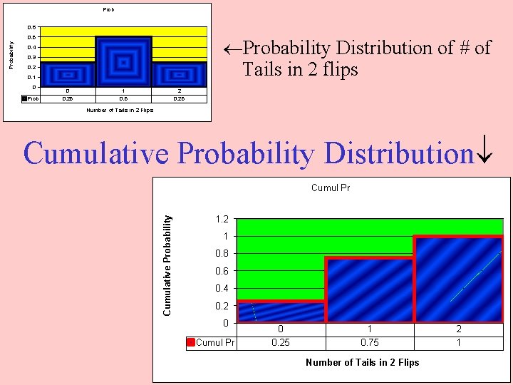
Prob 0. 6 Probability Distribution of # of Tails in 2 flips 0. 4 0. 3 0. 2 0. 1 0 Prob 0 0. 25 1 0. 5 2 0. 25 Number of Tails in 2 Flips Cumulative Probability Distribution Cumul Pr Cumulative Probability 0. 5 1. 2 1 0. 8 0. 6 0. 4 0. 2 0 Cumul Pr 0 0. 25 1 0. 75 Number of Tails in 2 Flips 2 1

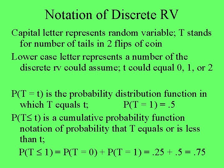
Notation of Discrete RV Capital letter represents random variable; T stands for number of tails in 2 flips of coin Lower case letter represents a number of the discrete rv could assume; t could equal 0, 1, or 2 P(T = t) is the probability distribution function in which T equals t; P(T = 1) =. 5 P(T t) is a cumulative probability function notation of probability that T equals or is less than t; P(T 1) = P(T = 0) + P(T = 1) =. 25 +. 5 =. 75

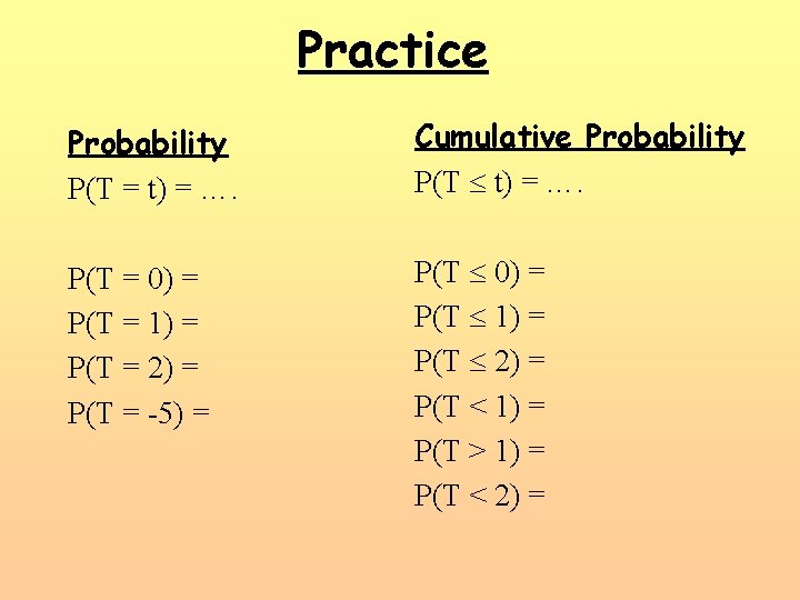
Practice Probability P(T = t) = …. Cumulative Probability P(T t) = …. P(T = 0) = P(T = 1) = P(T = 2) = P(T = -5) = P(T 0) = P(T 1) = P(T 2) = P(T < 1) = P(T > 1) = P(T < 2) =

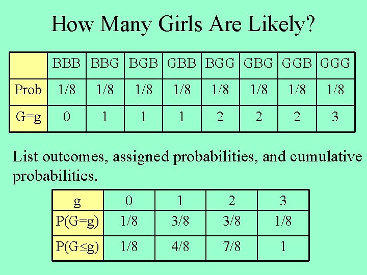
How Many Girls Are Likely? BBB BBG BGB GBB BGG GBG GGB GGG Prob 1/8 1/8 G=g 0 1 1 1 2 2 2 3 List outcomes, assigned probabilities, and cumulative probabilities. g P(G=g) 0 1/8 1 3/8 2 3/8 3 1/8 P(G g) 1/8 4/8 7/8 1

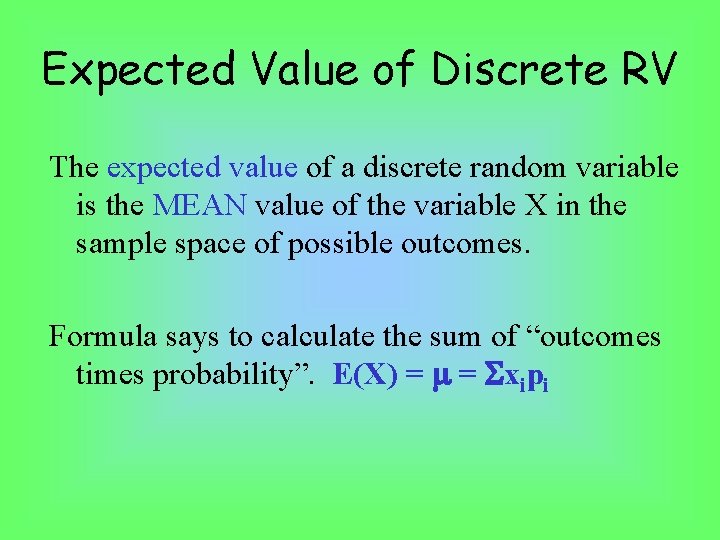
Expected Value of Discrete RV The expected value of a discrete random variable is the MEAN value of the variable X in the sample space of possible outcomes. Formula says to calculate the sum of “outcomes times probability”. E(X) = = xipi

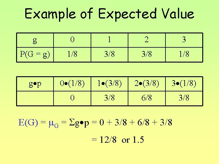
Example of Expected Value g 0 1 2 3 P(G = g) 1/8 3/8 1/8 g p 0 (1/8) 1 (3/8) 2 (3/8) 3 (1/8) 0 3/8 6/8 3/8 E(G) = G = g p = 0 + 3/8 + 6/8 + 3/8 = 12/8 or 1. 5

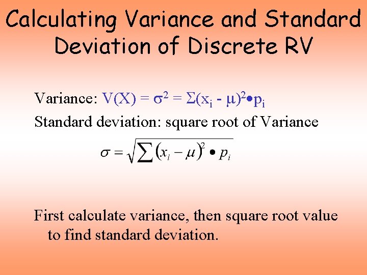
Calculating Variance and Standard Deviation of Discrete RV Variance: V(X) = 2 = (xi - )2 pi Standard deviation: square root of Variance First calculate variance, then square root value to find standard deviation.

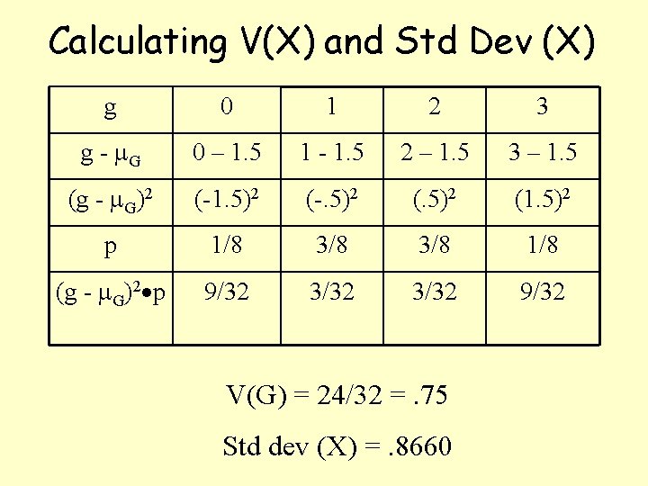
Calculating V(X) and Std Dev (X) g 0 1 2 3 g - G 0 – 1. 5 1 - 1. 5 2 – 1. 5 3 – 1. 5 (g - G)2 (-1. 5)2 (-. 5)2 (1. 5)2 p 1/8 3/8 1/8 (g - G)2 p 9/32 3/32 9/32 V(G) = 24/32 =. 75 Std dev (X) =. 8660

Using the TI-83+ to Calculate µ and Click here! • Put the values of the X into L 1 • Put the P(X=x) into L 2 • Choose 1 Var-Stats input L 1 and L 2 – 1 Var-Stats L 1, L 2 • The output lists the expected value as x and the standard deviation as .

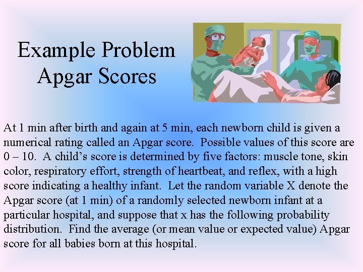
Example Problem Apgar Scores At 1 min after birth and again at 5 min, each newborn child is given a numerical rating called an Apgar score. Possible values of this score are 0 – 10. A child’s score is determined by five factors: muscle tone, skin color, respiratory effort, strength of heartbeat, and reflex, with a high score indicating a healthy infant. Let the random variable X denote the Apgar score (at 1 min) of a randomly selected newborn infant at a particular hospital, and suppose that x has the following probability distribution. Find the average (or mean value or expected value) Apgar score for all babies born at this hospital.

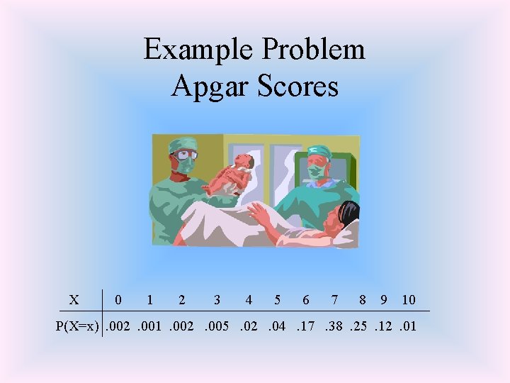
Example Problem Apgar Scores X 0 1 2 3 4 5 6 7 8 9 10 P(X=x). 002. 001. 002. 005. 02. 04. 17. 38. 25. 12. 01

Continuous Random Variable Probabilities of continuous random variables equals the proportion of area shaded under the curve. The total area under the curve is equal to 1.

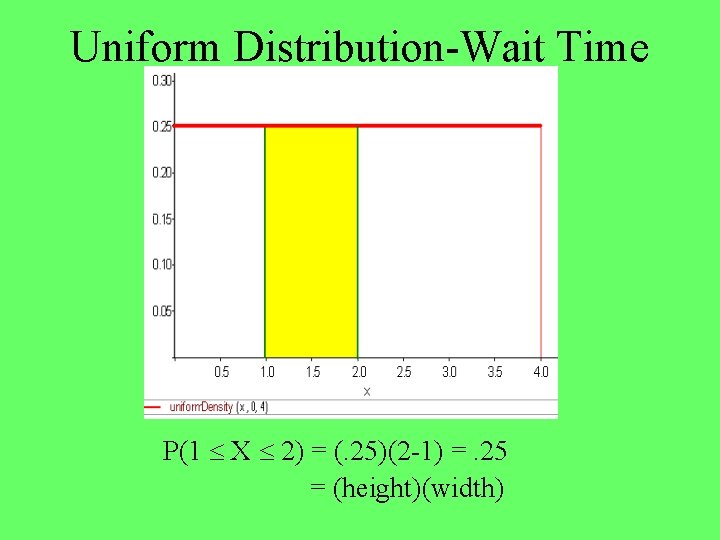
Uniform Distribution-Wait Time P(1 X 2) = (. 25)(2 -1) =. 25 = (height)(width)

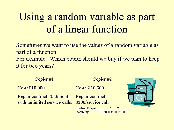
Using a random variable as part of a linear function Sometimes we want to use the values of a random variable as part of a function. For example: Which copier should we buy if we plan to keep it for two years? Copier #1 Cost: $10, 000 Copier #2 Cost: $10, 500 Repair contract: $50/month Repair contract: with unlimited service calls. $200/service call Number of Repairs Probability 0 1 2 0. 50 0. 25 0. 15 3 0. 10

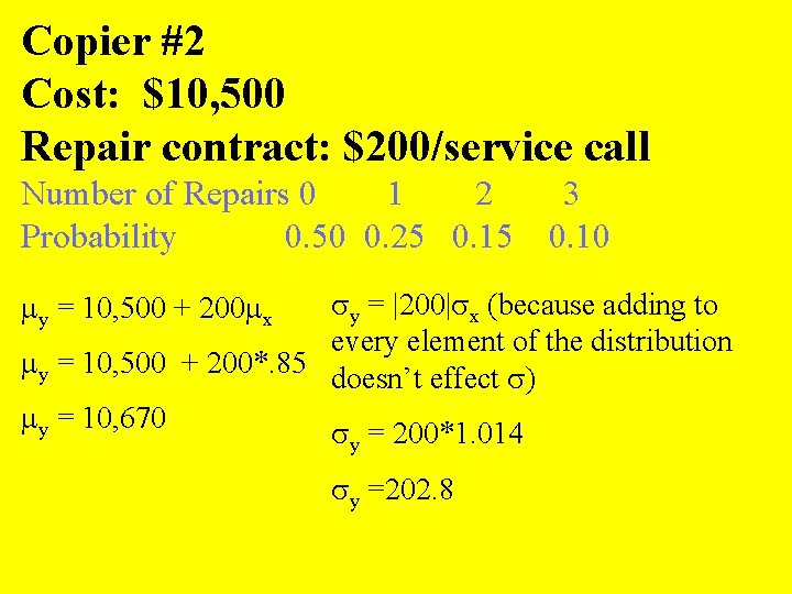
Copier #2 Cost: $10, 500 Repair contract: $200/service call Number of Repairs 0 1 2 Probability 0. 50 0. 25 0. 15 3 0. 10 y = |200| x (because adding to every element of the distribution y = 10, 500 + 200*. 85 doesn’t effect ) y = 10, 670 y = 200*1. 014 y = 10, 500 + 200 x y =202. 8

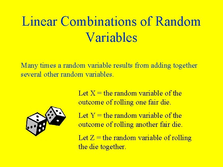
Linear Combinations of Random Variables Many times a random variable results from adding together several other random variables. Let X = the random variable of the outcome of rolling one fair die. Let Y = the random variable of the outcome of rolling another fair die. Let Z = the random variable of rolling the die together.

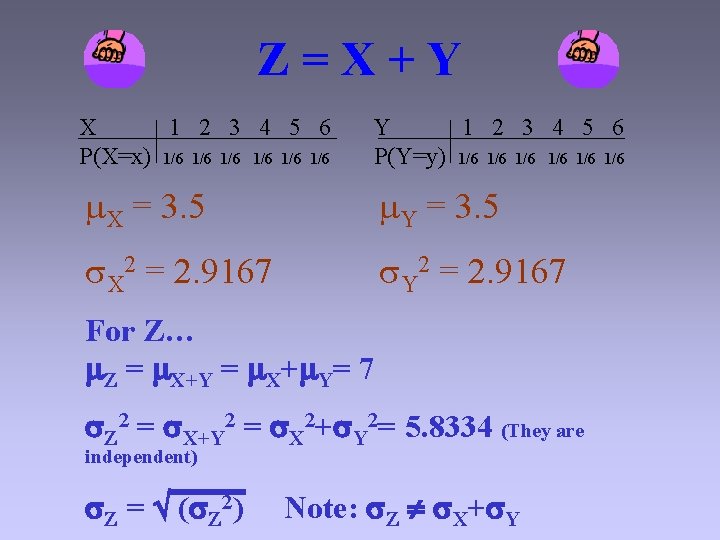
Z=X+Y X 1 2 3 4 5 6 P(X=x) 1/6 1/6 1/6 Y 1 2 3 4 5 6 P(Y=y) 1/6 1/6 1/6 X = 3. 5 Y = 3. 5 X 2 = 2. 9167 Y 2 = 2. 9167 For Z… Z = X+Y = X+ Y= 7 Z 2 = X+Y 2 = X 2+ Y 2= 5. 8334 (They are independent) Z = ( Z 2) Note: Z X+ Y

2010 AP Exam (Form B) A test consisting of 25 multiple-choice questions with 5 answer choices for each question is administered. For each question, there is only 1 correct answer. Let X be the number of correct answers if a student guesses randomly from the 5 choices for each of the 25 questions. What is the probability distribution of X ?

2011 AP Exam (Form B) An airline claims that there is a 0. 10 probability that a coach-class ticket holder who flies frequently will be upgraded to first class on any flight. This outcome is independent from flight to flight. Sam is a frequent flier who always purchases coach-class tickets. What is the probability that Sam’s first upgrade will occur after the third flight? What is the probability that Sam will be upgraded exactly 2 times in his next 20 flights? Sam will take 104 flights next year. Would you be surprised if Sam receives more than 20 upgrades to first class during the year? Justify your answer.

Binomial and Geometric Distributions • Binomial Distribution – Only two possible outcomes per trial – Fixed number of trials – Each trial is independent of the others – The probability of success remains constant • Geometric Distribution – Only two possible outcomes per trial – Each trial is independent of the others – The probability of success remains constant

What about sampling without replacement? When you sample without replacement from a population the trials are not independent. The probability is not remaining constant for each trial. So, it isn’t a binomial experiment. However… If the sample size, n, is less than 5% of the population size, N, then you can treat it as though the trials are independent even when sampling without replacement. The change in probability from one trial to the next is negligible. In this case a binomial distribution is still a good model.

Binomial or Geometric? • The number of LCD TVs sold out of the next 8 TVs sold at an electronics store. • The number of girls that must be asked to get a date to prom. • The number of plays that must be run to score a touchdown. • The number of face cards drawn in a 5 card poker hand. Remember to check for independence!

Binomial or Geometric? • The number of LCD TVs sold out of the next 8 TVs sold at an electronics store. • The number of girls that must be asked to get a date to prom. • The number of plays that must be run to score a touchdown. • The number of face cards drawn in a 5 card poker hand. Remember to check for independence!

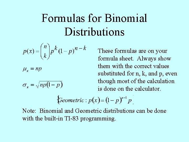
Formulas for Binomial Distributions These formulas are on your formula sheet. Always show them with the correct values substituted for n, k, and p, even though most of the calculation is done on the calculator. Note: Binomial and Geometric distributions can be done with the built-in TI-83 programming.

On the SAT, there are five answer choices (A, B, C, D, and E). The probability of randomly guessing the correct answer is. 2. What is the probability that on a 25 -question section of the SAT by complete random guessing that exactly 8 questions will be answered correctly? What is the probability that on a 25 -question section of the SAT by complete random guessing that 6 or fewer questions will be answered correctly? What is the probability that on a 25 -question section of the SAT by complete random guessing that the first correctly guessed answered is the fourth? What is the probability that on a 25 -question section of the SAT by complete random guessing that the first correct answer will be within the first 6 guesses? What is the expected number of correct guesses on a 25 -question section of the SAT exam

On the SAT, there are five answer choices (A, B, C, D, and E). The probability of randomly guessing the correct answer is. 2. 1. There are only two possible outcomes per trial: A correct guess or an incorrect guess. 2. The probability of guessing right stays 1/5 for every trial. 3. Since the selections are random the outcome of one trial doesn’t influence the outcome of any other trial. 4. Some of the problems represent a fixed number of trials (answering all 25 questions and examining the results), and some do not (seeing how many questions must be answered to achieve a desired outcome).

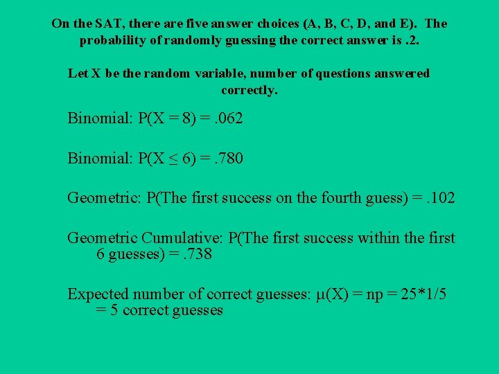
On the SAT, there are five answer choices (A, B, C, D, and E). The probability of randomly guessing the correct answer is. 2. Let X be the random variable, number of questions answered correctly. Binomial: P(X = 8) =. 062 Binomial: P(X ≤ 6) =. 780 Geometric: P(The first success on the fourth guess) =. 102 Geometric Cumulative: P(The first success within the first 6 guesses) =. 738 Expected number of correct guesses: µ(X) = np = 25*1/5 = 5 correct guesses

Major universities claim that 72% of their senior athletes graduate that year. Fifty senior athletic students attending major universities are randomly selected and recorded in order of selection. What is the probability that exactly 40 senior athletic students graduate that year? What is the probability that 40 or 41 or 42 senior athletic students graduated that year? What is the probability that 40 or fewer senior athletic students graduated that year? What is the probability that 41 or more senior athletic students graduated that year? What is the probability that 40 or more senior athletic students graduated that year? What is the probability that the first senior athletic student to graduate in the group of 50 that year is the 5 th selected?

Major universities claim that 72% of their senior athletes graduate that year. Fifty senior athletic students attending major universities are randomly selected and recorded in order of selection. 1. There are only two possible outcomes for each senior athlete, graduating or not graduating. 2. The trials are independent: Since the athletes are selected at random, whether one senior graduates or not does not affect the graduation status of the next selected athlete. 3. The probability does not remain constant b/c the athletes are selected without replacement. However it is reasonable to conclude that 50 senior athletes is less than or equal to 5% of the entire population of senior athletes from all major universities. 4. The situations in which we select all fifty athletes and then examine the results are binomial (fixed number of trials). Those in which we select senior athletes until a desired result is achieved are geometric (no fixed number of trials).

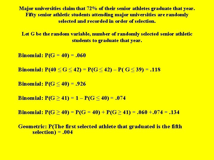
Major universities claim that 72% of their senior athletes graduate that year. Fifty senior athletic students attending major universities are randomly selected and recorded in order of selection. Let G be the random variable, number of randomly selected senior athletic students to graduate that year. Binomial: P(G = 40) =. 060 Binomial: P(40 ≤ G ≤ 42) = P(G ≤ 42) – P( G ≤ 39) =. 118 Binomial: P(G ≤ 40) =. 926 Binomial: P(G ≥ 41) = 1 – P(G ≤ 40) =. 074 Binomial: P(G ≥ 40) = P(G = 40) + P(G ≥ 41) =. 060 +. 074 =. 134 Geometric: P(The first selected athlete that graduated is the fifth selection) =. 004

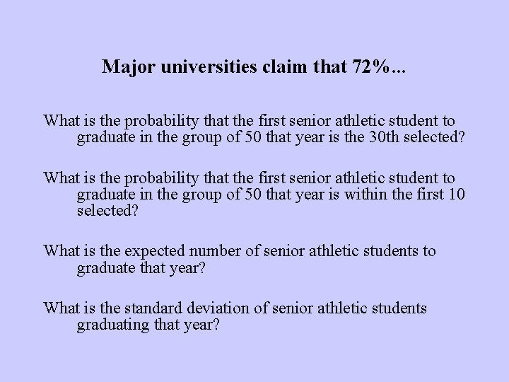
Major universities claim that 72%. . . What is the probability that the first senior athletic student to graduate in the group of 50 that year is the 30 th selected? What is the probability that the first senior athletic student to graduate in the group of 50 that year is within the first 10 selected? What is the expected number of senior athletic students to graduate that year? What is the standard deviation of senior athletic students graduating that year?

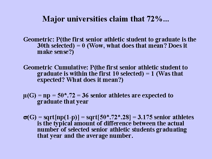
Major universities claim that 72%. . . Geometric: P(the first senior athletic student to graduate is the 30 th selected) = 0 (Wow, what does that mean? Does it make sense? ) Geometric Cumulative: P(the first senior athletic student to graduate is within the first 10 selected) = 1 (Was that expected? What does it mean? ) µ(G) = np = 50*. 72 = 36 senior athletes are expected to graduate that year (G) = sqrt[np(1 -p)] = sqrt[50*. 72*. 28] = 3. 175 senior athletes is the typical amount of difference between the actual number of selected senior athletic students graduating that year and the average number.

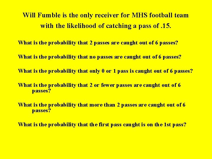
Will Fumble is the only receiver for MHS football team with the likelihood of catching a pass of. 15. What is the probability that 2 passes are caught out of 6 passes? What is the probability that no passes are caught out of 6 passes? What is the probability that only 0 or 1 pass is caught out of 6 passes? What is the probability that 2 or fewer passes are caught out of 6 passes? What is the probability that more than 2 passes are caught out of 6 passes? What is the probability that the first pass caught is on the 1 st pass?

Will Fumble is the only receiver for MHS football team with the likelihood of catching a pass of. 15. 1. There are only two possible outcomes per trial: Either Will catches the pass or he doesn’t. 2. We must assume that we are randomly selecting the pass attempts and that whether or not Will catches one pass has no bearing on the result of the next pass attempt selected. 3. We must assume that Will never improves or gets worse at catching passes so that the probability of catching a pass remains constant. 4. Some of the problems are binomial b/c we are examing the results of all 6 passes (fixed number of trials), others are geometric because we are examining results as soon as certain conditions are met (no fixed number of trials).

Will Fumble is the only receiver for MHS football team with the likelihood of catching a pass of. 15. Let C be the random variable, number of randomly selected pass attempts to Will that were completions. Binomial: P(C = 2) =. 176 Binomial: P(C = 0) =. 377 (Does this number seem too high? ) Binomial: P(C = 0 or 1) = P(C = 0) + P(C = 1) =. 776 Binomial: P(C = 2 or fewer) =. 776 +. 176 =. 952 Binomial: P(C = more than 2 caught) = 1 –. 952 =. 048 Geometric: P(The first pass caught is the first pass) =. 15 (This should have been obvious! Why? )

Will Fumble is the only receiver for MHS football team with the likelihood of catching a pass of . 15. Geometric: P(The first pass caught is on the 4 th pass) =. 092 Geometric Cumulative: P(The first pass is caught within the first 3 attempts) =. 386 Geometric Cumulative: P(The first pass is caught after the first 3 attempts) = 1 - P(The first pass is caught within the first 3 attempts) = 1 -. 386 =. 614 µ(C) = np = 6*. 15 =. 9 catches is the expect number of catches with 6 attempts µ(Number of attempts required for first catch) = 1/p = 1/. 15 = 6. 667 attempts is the expect number of attempts required for the first pass caught

2010 AP Exam (Form B) A test consisting of 25 multiple-choice questions with 5 answer choices for each question is administered. For each question, there is only 1 correct answer. Let X be the number of correct answers if a student guesses randomly from the 5 choices for each of the 25 questions. What is the probability distribution of X ?

2011 AP Exam (Form B) An airline claims that there is a 0. 10 probability that a coach-class ticket holder who flies frequently will be upgraded to first class on any flight. This outcome is independent from flight to flight. Sam is a frequent flier who always purchases coach-class tickets. What is the probability that Sam’s first upgrade will occur after the third flight? What is the probability that Sam will be upgraded exactly 2 times in his next 20 flights? Sam will take 104 flights next year. Would you be surprised if Sam receives more than 20 upgrades to first class during the year? Justify your answer.

Normal Distributions “Z easiest kind of all!”

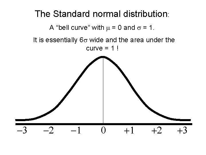
The Standard normal distribution: A “bell curve” with = 0 and = 1. It is essentially 6 wide and the area under the curve = 1 ! -3 -2 -1 0 +1 +2 +3

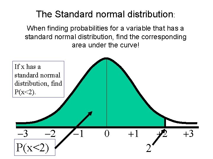
The Standard normal distribution: When finding probabilities for a variable that has a standard normal distribution, find the corresponding area under the curve! If x has a standard normal distribution, find P(x<2). -3 -2 P(x<2) -1 0 +1 +2 2 +3

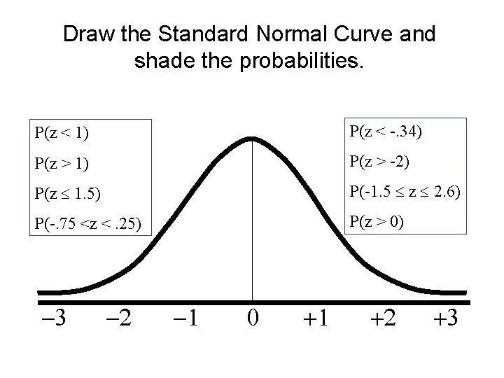
Draw the Standard Normal Curve and shade the probabilities. P(z < 1) P(z < -. 34) P(z > 1) P(z > -2) P(z 1. 5) P(-1. 5 z 2. 6) P(-. 75 <z <. 25) P(z > 0) -3 -2 -1 0 +1 +2 +3

Using Z-Table Find the two tables representing z-scores from – 3. 49 to +3. 49. Notice which direction the area under the curve is shaded (to the left). The assigned probabilities represents the area shaded under the curve from the z-score and far left of the z-score.

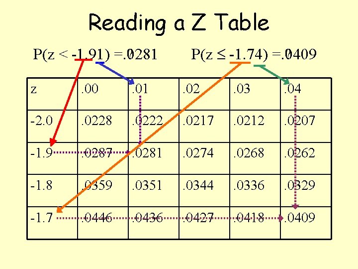
Reading a Z Table P(z < -1. 91) =. 0281 ? P(z -1. 74) =. 0409 ? z . 00 . 01 . 02 . 03 . 04 -2. 0 . 0228 . 0222 . 0217 . 0212 . 0207 -1. 9 . 0287 . 0281 . 0274 . 0268 . 0262 -1. 8 . 0359 . 0351 . 0344 . 0336 . 0329 -1. 7 . 0446 . 0436 . 0427 . 0418 . 0409

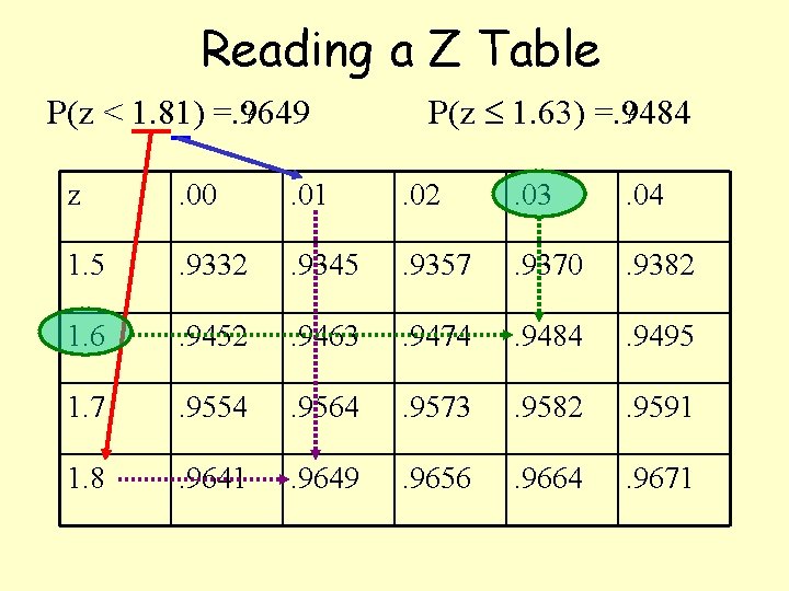
Reading a Z Table P(z < 1. 81) =. 9649 ? P(z 1. 63) =. 9484 ? z . 00 . 01 . 02 . 03 . 04 1. 5 . 9332 . 9345 . 9357 . 9370 . 9382 1. 6 . 9452 . 9463 . 9474 . 9484 . 9495 1. 7 . 9554 . 9564 . 9573 . 9582 . 9591 1. 8 . 9641 . 9649 . 9656 . 9664 . 9671

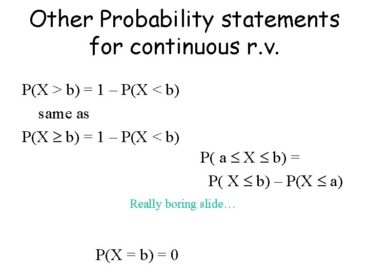
Other Probability statements for continuous r. v. P(X > b) = 1 – P(X < b) same as P(X b) = 1 – P(X < b) P( a X b) = P( X b) – P(X a) Really boring slide… P(X = b) = 0

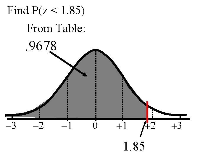
Find P(z < 1. 85) From Table: . 9678 -3 -2 -1 0 +1 +2 1. 85 +3

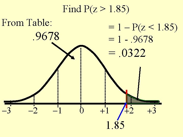
Find P(z > 1. 85) From Table: = 1 – P(z < 1. 85) = 1 -. 9678 =. 0322 -3 -2 -1 0 +1 +2 1. 85 +3

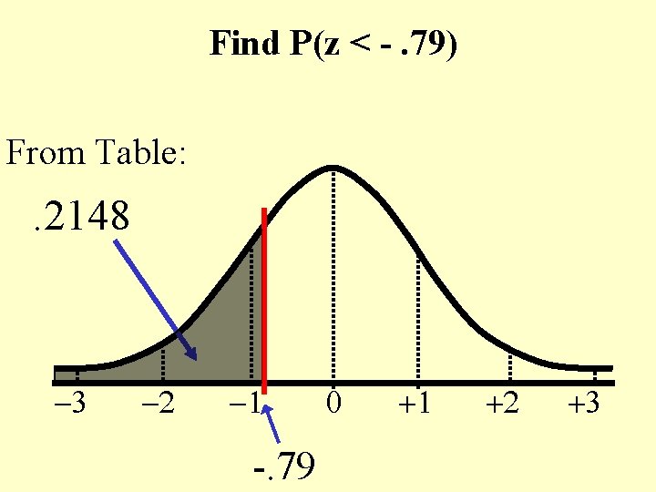
Find P(z < -. 79) From Table: . 2148 -3 -2 -1 -. 79 0 +1 +2 +3

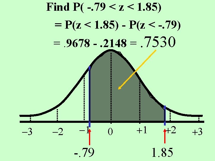
Find P( -. 79 < z < 1. 85) = P(z < 1. 85) - P(z < -. 79) =. 9678 -. 2148 =. 7530 -3 -2 -1 -. 79 0 +1 +2 1. 85 +3

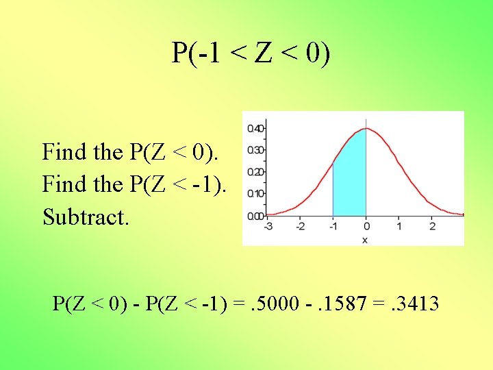
P(-1 < Z < 0) Find the P(Z < 0). Find the P(Z < -1). Subtract. P(Z < 0) - P(Z < -1) =. 5000 -. 1587 =. 3413

Non-standard Normal Distributions • Draw Normal Curve – Label mean – Label standard deviation • Plot the value(s) of x. • Shade the appropriate area. • Find the z-score(s) corresponding to the value(s) of x. • Find the probability. From the table or the calculator.

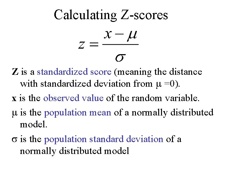
Calculating Z-scores Z is a standardized score (meaning the distance with standardized deviation from =0). x is the observed value of the random variable. is the population mean of a normally distributed model. is the population standard deviation of a normally distributed model

What is the probability that a randomly selected student scored below 73% on the Calculus exam if the grades were normally distributed with a mean of 78% and a standard deviation of 4%?

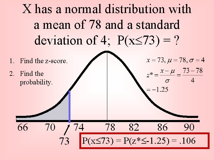
X has a normal distribution with a mean of 78 and a standard deviation of 4; P(x 73) = ? 1. Find the z-score. 2. Find the probability. 66 70 74 73 78 82 86 90 P(x 73) = P(z* -1. 25) =. 106

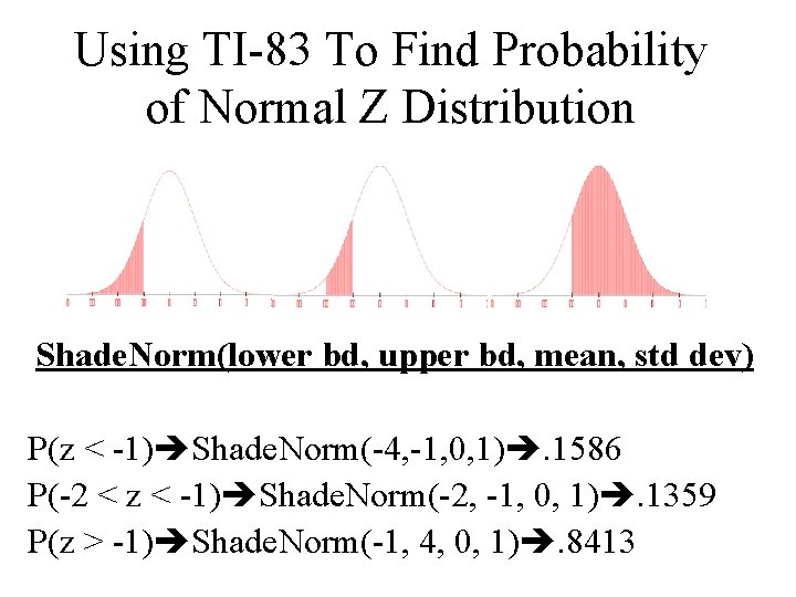
Using TI-83 To Find Probability of Normal Z Distribution Shade. Norm(lower bd, upper bd, mean, std dev) P(z < -1) Shade. Norm(-4, -1, 0, 1). 1586 P(-2 < z < -1) Shade. Norm(-2, -1, 0, 1). 1359 P(z > -1) Shade. Norm(-1, 4, 0, 1). 8413

Finding z when given P? What does it mean to score at the 80 th percentile on the SAT exam? How many standardized standard deviations from the mean was that SAT score? Would the number of standardized standard deviations (z-score) be positive or negative?

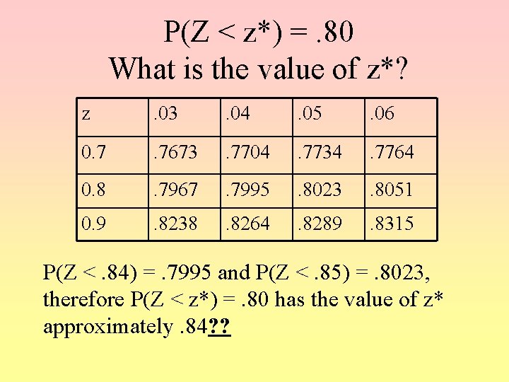
P(Z < z*) =. 80 What is the value of z*? z . 03 . 04 . 05 . 06 0. 7 . 7673 . 7704 . 7734 . 7764 0. 8 . 7967 . 7995 . 8023 . 8051 0. 9 . 8238 . 8264 . 8289 . 8315 P(Z <. 84) =. 7995 and P(Z <. 85) =. 8023, therefore P(Z < z*) =. 80 has the value of z* approximately. 84? ?

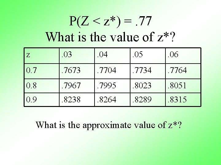
P(Z < z*) =. 77 What is the value of z*? z . 03 . 04 . 05 . 06 0. 7 . 7673 . 7704 . 7734 . 7764 0. 8 . 7967 . 7995 . 8023 . 8051 0. 9 . 8238 . 8264 . 8289 . 8315 What is the approximate value of z*?

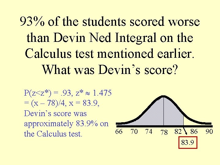
93% of the students scored worse than Devin Ned Integral on the Calculus test mentioned earlier. What was Devin’s score? P(z<z*) =. 93, z* 1. 475 = (x – 78)/4, x = 83. 9, Devin’s score was approximately 83. 9% on 66 70 74 78 82 86 90 the Calculus test. 83. 9

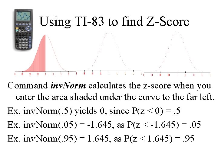
Using TI-83 to find Z-Score Command inv. Norm calculates the z-score when you enter the area shaded under the curve to the far left. Ex. inv. Norm(. 5) yields 0, since P(z < 0) =. 5 Ex. inv. Norm(. 05) = -1. 645, as P(z < -1. 645) =. 05 Ex. inv. Norm(. 95) = 1. 645, as P(z < 1. 645) =. 95

inv. Norm( ). 05 . 95 . 10 Ex. inv. Norm(. 95) = 1. 645, since P(z > 1. 645) =. 95 Ex. inv. Norm(. 05) = -1. 645, as P(z > -1. 645) =. 95 Ex. inv. Norm(. 90) = 1. 281, as P(z >1. 281) =. 10

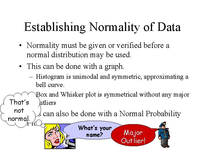
Establishing Normality of Data • Normality must be given or verified before a normal distribution may be used. • This can be done with a graph. – Histogram is unimodal and symmetric, approximating a bell curve. – Box and Whisker plot is symmetrical without any major That’s outliers not • This can also be done with a Normal Probability normal. Plot. What’s your name? Major Outlier!

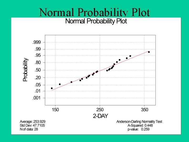
Normal Probability Plot

Transformations to Achieve Normality • If X is skewed left, – Square the data – Cube the data • See if the distribution of X 2 or X 3 is more normal. • If X is skewed right, – Square root the data – Cube root the data – Log or ln the data • See if the distribution of X, 3 X, log. X or ln. X is more normal.

Approximating a Binomial Distribution • A Binomial Distribution may be approximated using a normal distribution under certain conditions.

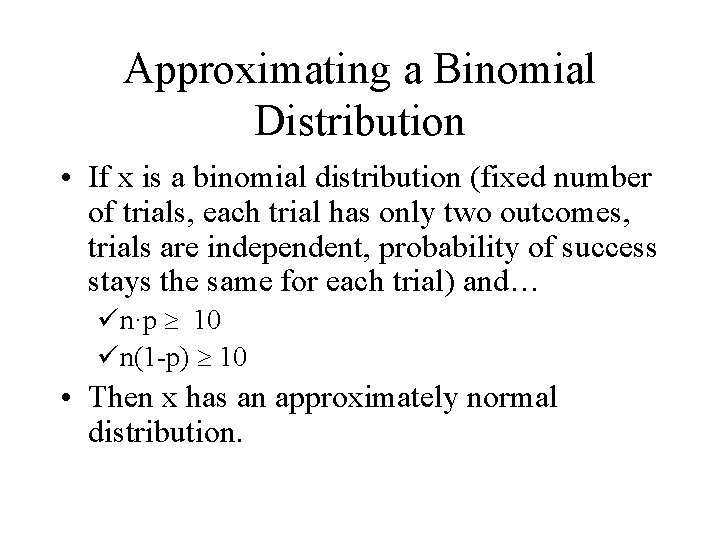
Approximating a Binomial Distribution • If x is a binomial distribution (fixed number of trials, each trial has only two outcomes, trials are independent, probability of success stays the same for each trial) and… ün·p 10 ün(1 -p) 10 • Then x has an approximately normal distribution.