Probability Distributions A Brief Introduction Normal Gaussian Distribution

Probability Distributions A Brief Introduction
 Distribution • Bell-shaped distribution with tendency for individuals to clump around the")
Normal (Gaussian) Distribution • Bell-shaped distribution with tendency for individuals to clump around the group median/mean • Used to model many biological phenomena • Many estimators have approximate normal sampling distributions (see Central Limit Theorem) • Notation: X~N(m, s 2) where m is mean and s 2 is variance Obtaining Probabilities and Quantiles in R: To obtain: F(x)=P(X≤x) Use Function: pnorm(x, m, s) To obtain the pth quantile: P(X≤xp)=p Use Function: qnorm(p, m, s) Virtually all statistics textbooks give the cdf (or upper tail probabilities) for standardized normal random variables: z=(x-m)/s ~ N(0, 1)
")
Normal Distribution – Density Functions (pdf)

Second Decimal Place of z Integer part and first decimal place of z
” X~cn 2 • Z~N(0, 1)")
Chi-Square Distribution • Indexed by “degrees of freedom (n)” X~cn 2 • Z~N(0, 1) Z 2 ~c 12 • Assuming Independence: Obtaining Probabilities in R: To obtain: 1 -F(x)=P(X≥x) Use Function: pchisq(x, n) To obtain quantiles: P(X≤xp)=p Use Function: qchisq(x, n) Virtually all statistics textbooks give upper tail cut-off values for commonly used upper (and sometimes lower) tail probabilities

Chi-Square Distributions
")
Critical Values for Chi-Square Distributions (Mean=n, Variance=2 n)
” X~tn • Z~N(0, 1), X~cn")
Student’s t-Distribution • Indexed by “degrees of freedom (n)” X~tn • Z~N(0, 1), X~cn 2 • Assuming Independence of Z and X: Obtaining Probabilities /Quantiles in R: To obtain: F(t)=P(T≤t) pt(t, n) To obtain: pth quantile: qt(p, n) Virtually all statistics textbooks give upper tail cut-off values for commonly used upper tail probabilities
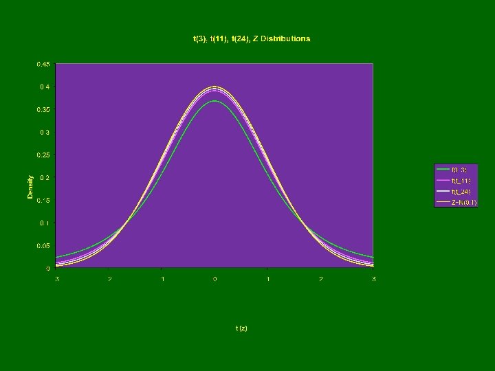

Critical Values for Student’s t-Distributions
” W~Fn 1,")
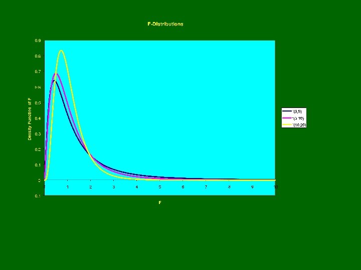
F-Distribution • Indexed by 2 “degrees of freedom (n 1, n 2)” W~Fn 1, n 2 • X 1 ~cn 12, X 2 ~cn 22 • Assuming Independence of X 1 and X 2: Obtaining Probabilities/Quantiles in R: To obtain: F(w)=P(W≤w): pf(w, n 1, n 2) pth quantile: qf(p, n 1, n 2) Virtually all statistics textbooks give upper tail cut-off values for commonly used upper tail probabilities
 = 0. 95")
Critical Values for F-distributions P(F ≤ Table Value) = 0. 95

Multivariate Normal Distribution

Results Involving Multivariate Normal - I

Results Involving Multivariate Normal - II

Results Involving Multivariate Normal - III

Results Involving Multivariate Normal - IV

Multivariate Normal Likelihood Function

Maximum Likelihood Estimator of m

Maximum Likelihood Estimator of S

Results for ML Estimators and Large-Sample Properties

Data – Heights of Adult Children and Parents • Adult Children Heights are reported by inch, in a manner so that the median of the grouped values is used for each (62. 2”, …, 73. 2” are reported by Galton). § He adjusts female heights by a multiple of 1. 08 § We use 61. 2” for his “Below” § We use 74. 2” for his “Above” • Mid-Parents Heights are the average of the two parents’ heights (after female adjusted). Grouped values at median (64. 5”, …, 72. 5” by Galton) § We use 63. 5” for “Below” § We use 73. 5” for “Above”


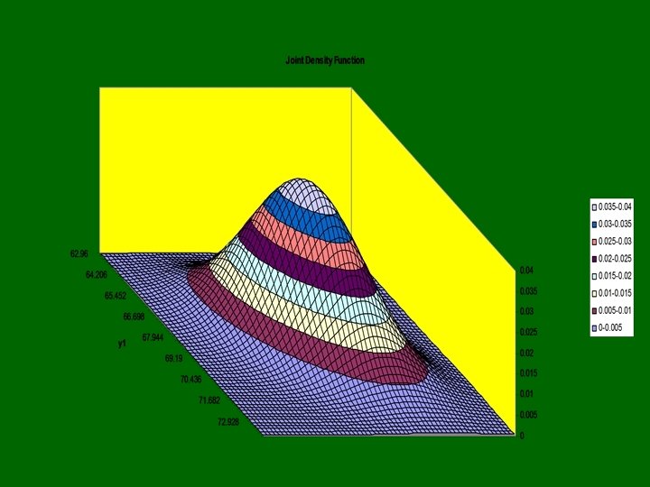
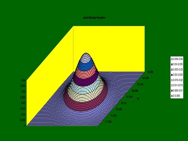
Joint Density Function m 1=m 2=0 s 1=s 2=1 r=0. 4
")
Marginal Distribution of X (p. 1)
")
Marginal Distribution of X (p. 2)
")
Conditional Distribution of X 2 Given X 1=x 1 (P. 1)
 This is referred")
Conditional Distribution of X 2 Given X 1=x 1 (P. 2) This is referred to as the REGRESSION of X 2 on X 1

Summary of Results

Heights of Adult Children and Parents • Empirical Data Based on 924 pairs (F. Galton) • X 2 = Adult Child’s Height – X 2 ~ N(68. 1, 6. 39) s 2=2. 53 • X 1 = Mid-Parent’s Height – X 1 ~ N(68. 3, 3. 18) s 1=1. 78 • COV(X 1, X 2) = 2. 02 r = 0. 45, r 2 = 0. 20 • X 2|X 1=x 1 is Normal with conditional mean and variance: Unconditional 63. 5 66. 5 69. 5 72. 5 E[X 2|x 1] 68. 1 65. 0 66. 9 68. 8 70. 8 s. X 2|x 1 2. 53 2. 26 x 1

= Parent+constant Galton’s Finding E(Child) independent of parent")
E(Child)= Parent+constant Galton’s Finding E(Child) independent of parent

Expectations and Variances E{X 1} = 68. 3 V{X 1} = 3. 18 E{X 2} = 68. 1 V{X 2} = 6. 39 E{X 2|X 1=x 1} = 24. 5+0. 638 x 1 EX 1[E{X 2|X 1=x 1}] = EX 1[24. 5+0. 638 X 1] = 24. 5+0. 638(68. 3) = 68. 1 = E{X 2} • V{X 2|X 1=x 1} = 5. 11 EX 1[V{X 2|X 1=x 1}] = 5. 11 • VX 1[E{X 2|X 1=x 1}] = VX 1[24. 5+0. 638 X 1] = (0. 638)2 V(X 1) = (0. 407)3. 18 = 1. 29 • EX 1[V{X 2|X 1=x 1}]+VY 1[E{X 2|X 1=x 1}] = 5. 11+1. 29=6. 40 = V(X 2) (with round-off) • •
- Slides: 38